Cloudera Databricks Data Science Certification Questions and Answers (Dumps and Practice Questions)

Question : PCA analyzes the all the variance in the in the variables and reorganizes it into a new set of
components equal to the number of original variables. Regarding these new variables which of the following statement are correct?

1. They are independent
2. They decrease in the amount of variance in the originals they account for First component captures most of the variance, 2ndsecond most and so on until all the variance is accounted for
3. Access Mostly Uused Products by 50000+ Subscribers
4. Only 1 and 3
5. All 1,2 and 3


Correct Answer : Get Lastest Questions and Answer :
Conceptually the goal of PCA is to reduce the number of variables of interest into a smaller set of components.
PCA analyzes the all the variance in the in the variables and reorganizes it into a new set of components equal to the number of original variables.

Regarding the new components:
- They are independent
- They decrease in the amount of variance in the originals they account forFirst component captures most of the variance, 2ndsecond most and so on until all the variance is accounted for
- Only some will be retained for further study (dimension reduction)Since the first few capture most of the variance they are typically of focus






Question : PCA is a parametric method of extracting relevant information form confusing data sets.



1. True
2. False

Correct Answer : Get Lastest Questions and Answer :

Principal component analysis (PCA) has been called one of the most valuable results from applied linear algebra. PCA is used abundantly in all forms of analysis - from neuroscience to computer graphics - because it is a simple, non-parametric method of extracting relevant information from confusing data sets. With minimal additional effort PCA provides a roadmap for how to reduce a complex data set to a lower dimension to reveal the sometimes hidden, simplified dynamics that often underlie it.






Question : In Supervised Learning you have performed the following steps
1. Determine the type of training examples
2. Gather a training set. The training set needs to be representative of the real-world use of the function
3. Access Mostly Uused Products by 50000+ Subscribers
4. Determine the structure of the learned function and corresponding learning algorithm,
5. Complete the design. Run the learning algorithm on the gathered training set
6.Evaluate the accuracy of the learned function.

In the 4th step which of the following algorithm you can apply



1. Support Vector Machine
2. Decision trees
3. Access Mostly Uused Products by 50000+ Subscribers
4. 1 and 2 only
5. All 1,2 and 3


Correct Answer : Get Lastest Questions and Answer :
In order to solve a given problem of supervised learning, one has to perform the following steps:

1.Determine the type of training examples. Before doing anything else, the user should decide what kind of data is to be used as a training set. In the case of handwriting analysis, for example, this might be a single handwritten character, an entire handwritten word, or an entire line of handwriting.
2.Gather a training set. The training set needs to be representative of the real-world use of the function. Thus, a set of input objects is gathered and corresponding outputs are also gathered, either from human experts or from measurements.
3. Access Mostly Uused Products by 50000+ Subscribers
4.Determine the structure of the learned function and corresponding learning algorithm. For example, the engineer may choose to use support vector machines or decision trees.
5.Complete the design. Run the learning algorithm on the gathered training set. Some supervised learning algorithms require the user to determine certain control parameters. These parameters may be adjusted by optimizing performance on a subset (called a validation set) of the training set, or via cross-validation.
6.Evaluate the accuracy of the learned function. After parameter adjustment and learning, the performance of the resulting function should be measured on a test set that is separate from the training set.

Related Questions

---

Question :Select the correct Hive function which will Returns the population covariance of a pair of numeric columns in the group.


1. covar_pop(col1, col2)
2. corr(col1, col2)
3. Access Mostly Uused Products by 50000+ Subscribers
4. 1 and 2
5. All 1,2 and 3




Question : Which of the following Hive function Returns the standard deviation of a numeric column in the group


1. stddev_pop(col)
2. stddev_samp(col)
3. Access Mostly Uused Products by 50000+ Subscribers
4. dev_pop(col)





Question : You have two tables in Hive that are populated with data:
Employee
emp_id int
salary string

Employee_Detail;
emp_id int
name string

You now create a new table de-normalized one and populate it with the results of joining the two tables as follows:
CREATE TABLE EMPLOYEE_FULL AS SELECT Employee_Detail.*,Employee.salary AS s
FROM Employee JOIN Employee_Detail ON (Employee.emp_id== Employee_Detail.emp_id);

You then export the table and download the file:
EXPORT TABLE EMPLOYEE_FULL TO '/hadoopexam/employee/Employee_Detail.data';

You have downloaded the file and read the file as a CSV in R. How many columns will the resulting variable in R have?





1. 1
2. 2
3. Access Mostly Uused Products by 50000+ Subscribers
4. 4
5. 5

Ans : 1
Exp :The Stinger Initiative successfully delivered a fundamental new Apache Hive, which evolved Hive's traditional architecture and made it faster, with richer SQL semantics and petabyte scalability. We continue to work within the community to advance these three key facets of hive: Speed Deliver sub-second query response times. Scale : The only SQL interface to Hadoop designed for queries that scale from Gigabytes, to Terabytes and Petabytes
SQL : Enable transactions and SQL:2011 Analytics for Hive
Stinger.next is focused on the vision of delivering enterprise SQL at Hadoop scale, accelerating the production deployment of Hive for interactive analytics, reporting and and ETL. More explicitly, some of the key areas that we will invest in include: When exporting a table from Hive, the data file will use the delimiters form the table. Because table3 wasn't created with specific delimiters, it will use the default Hive delimiter, which is \001 or Control-A. When the file is imported into R as a CSV, there will be only 1 column because the file isn't actually comma delimited.adoop was built to organize and store massive amounts of data of all shapes, sizes and formats. Because of Hadoop's "schema on read" architecture, a Hadoop cluster is a perfect reservoir of heterogeneous data-structured and unstructured-from a multitude of sources. Data analysts use Hive to explore, structure and analyze that data, then turn it into business insight.
Here are some advantageous characteristics of Hive for enterprise SQL in Hadoop:
Feature Description, Familiar , Query data with a SQL-based language , Fast Interactive response times, even over huge datasets Scalable and Extensible
As data variety and volume grows, more commodity machines can be added, without a corresponding reduction in performance. The tables in Hive are similar to tables in a relational database, and data units are organized in a taxonomy from larger to more granular units. Databases are comprised of tables, which are made up of partitions. Data can be accessed via a simple query language and Hive supports overwriting or appending data. Within a particular database, data in the tables is serialized and each table has a corresponding Hadoop Distributed File System (HDFS) directory. Each table can be sub-divided into partitions that determine how data is distributed within sub-directories of the table directory. Data within partitions can be further broken down into buckets. Hive supports all the common primitive data formats such as BIGINT, BINARY, BOOLEAN, CHAR, DECIMAL, DOUBLE, FLOAT, INT, SMALLINT, STRING, TIMESTAMP, and TINYINT. In addition, analysts can combine primitive data types to form complex data types, such as structs, maps and arrays.




Question :You have a HadoopExam Log files directory containing a number of comma files.
Each of the files has three columns and each of the filenames has a .log extension like 12012014.log, 13012014.log, 14012014.log etc.
You want a single comma-separated file (with extension .csv) that contains all the rows from
all the files that do not contain the word "HadoopExam", case-sensitive.

1. cat *.log | grep -v HadoopExam > final.csv
2. find . -name '*.log' -print0 | xargs -0 cat | awk 'BEGIN {print $1, $2, $3}' | grep -v HadoopExam > final.csv
3. Access Mostly Uused Products by 50000+ Subscribers
4. grep HadoopExam *.log > final.csv


Ans: 2
Exp : There are three variations of AWK: AWK - the (very old) original from AT&T NAWK - A newer, improved version from AT&T
GAWK - The Free Software foundation's version , The essential organization of an AWK program follows the form: pattern { action }
The pattern specifies when the action is performed. Like most UNIX utilities, AWK is line oriented. That is, the pattern specifies a test that is performed with each line read as input. If the condition is true, then the action is taken. The default pattern is something that matches every line. This is the blank or null pattern. Two other important patterns are specified by the keywords "BEGIN" and "END". As you might expect, these two words specify actions to be taken before any lines are read, and after the last line is read. The AWK program below:
BEGIN { print "START" } { print } END { print "STOP" }
adds one line before and one line after the input file. This isn't very useful, but with a simple change, we can make this into a typical AWK program:
BEGIN { print "File\tOwner"} { print $8, "\t", $3} END { print " - DONE -" } I'll improve the script in the next sections, but we'll call it "FileOwner". But let's not put it into a script or file yet. I will cover that part in a bit. Hang on and follow with me so you get the flavor of AWK. The characters "\t" Indicates a tab character so the output lines up on even boundries. The "$8" and "$3" have a meaning similar to a shell script. Instead of the eighth and third argument, they mean the eighth and third field of the input line. You can think of a field as a column, and the action you specify operates on each line or row read in. There are two differences between AWK and a shell processing the characters within double quotes. AWK understands special characters follow the "\" character like "t". The Bourne and C UNIX shells do not. Also, unlike the shell (and PERL) AWK does not evaluate variables within strings. To explain, the second line could not be written like this: {print "$8\t$3" } That example would print "$8 $3". Inside the quotes, the dollar sign is not a special character. Outside, it corresponds to a field. What do I mean by the third and eight field? Consider the Solaris "/usr/bin/ls -l" command, which has eight columns of information. The System V version (Similar to the Linux version), "/usr/5bin/ls -l" has 9 columns. The third column is the owner, and the eighth (or nineth) column in the name of the file. This AWK program can be used to process the output of the "ls -l" command, printing out the filename, then the owner, for each file. I'll show you how. Update: On a linux system, change "$8" to "$9". One more point about the use of a dollar sign. In scripting languages like Perl and the various shells, a dollar sign means the word following is the name of the variable. Awk is different. The dollar sign means that we are refering to a field or column in the current line. When switching between Perl and AWK you must remener that "$" has a different meaning. So the following piece of code prints two "fields" to standard out. The first field printed is the number "5", the second is the fifth field (or column) on the input line. BEGIN { x=5 } { print x, $x}
Originally, I didn't plan to discuss NAWK, but several UNIX vendors have replaced AWK with NAWK, and there are several incompatibilities between the two. It would be cruel of me to not warn you about the differences. So I will highlight those when I come to them. It is important to know than all of AWK's features are in NAWK and GAWK. Most, if not all, of NAWK's features are in GAWK. NAWK ships as part of Solaris. GAWK does not. However, many sites on the Internet have the sources freely available. If you user Linux, you have GAWK. But in general, assume that I am talking about the classic AWK unless otherwise noted.
You can only specify a small number of files to a command like cat, so globbing 100,000 files will cause an error. In this instance, you must use find and xargs. The grep flag should be -v to invert the sense of matching. The -i ignores the case. You switch the delimiter with awk, though tr works also.





Question : In recommender systems, the ___________ problem is often reduced by adopting a hybrid approach
between content-based matching and collaborative filtering. New items (which have not yet received any
ratings from the community) would be assigned a rating automatically, based on the ratings assigned by
the community to other similar items. Item similarity would be determined according to the items' content-based characteristics.



1. hot-start
2. cold start
3. Access Mostly Uused Products by 50000+ Subscribers
4. Automated rating
Ans : 2
Exp :






Question : The cold start" problem happens in recommendation systems due to


1. Huge volume of data to analyze
2. Very small amount of data to analyze
3. Access Mostly Uused Products by 50000+ Subscribers
4. Information is enough but less memory
Ans :3
Exp : The cold start" problem happens in recommendation systems due to the lack of information, on users or items.






Question : Select the correct statement which applies to Collaborative filtering


1. Make recommendation based on past user-item interaction
2. Better performance for old users and old items
3. Access Mostly Uused Products by 50000+ Subscribers
4. 1 and 2 are correct
5. All 1,2 and 3 are correct


Ans : 5
Exp : Collaborative filtering (CF aka Memory based)
Make recommendation based on past user-item interaction
Better performance for old users and old items
Does not naturally handle new users and new items








Question : You are creating a model for the recommending the book at Amazon.com, so which of the following
recommender system you will use you don't have cold start problem?


1. Naive Bayes classifier
2. K-Means Clustring
3. Access Mostly Uused Products by 50000+ Subscribers
4. Content-based filtering
Ans : 4
Exp : The cold start problem is most prevalent in recommender systems. Recommender systems form a specific type of information filtering (IF) technique that attempts to present information items (movies, music, books, news, images, web pages) that are likely of interest to the user. Typically, a recommender system compares the user's profile to some reference characteristics. These characteristics may be from the information item (the content-based approach) or the user's social environment (the collaborative filtering approach). In the content-based approach, the system must be capable of matching the characteristics of an item against relevant features in the user's profile. In order to do this, it must first construct a sufficiently-detailed model of the user's tastes and preferences through preference elicitation. This may be done either explicitly (by querying the user) or implicitly (by observing the user's behaviour). In both cases, the cold start problem would imply that the user has to dedicate an amount of effort using the system in its 'dumb' state - contributing to the construction of their user profile - before the system can start providing any intelligent recommendations. Content-based filtering recommender systems use information about items or users to make recommendations, rather than user preferences, so it will perform well with little user preference data. Item-based and user-based collaborative filtering makes predictions based on users' preferences for items, os they will typically perform poorly with little user preference data. Logistic regression is not recommender system technique. Content-based filtering, also referred to as cognitive filtering, recommends items based on a comparison between the content of the items and a user profile. The content of each item is represented as a set of descriptors or terms, typically the words that occur in a document. The user profile is represented with the same terms and built up by analyzing the content of items which have been seen by the user.
Several issues have to be considered when implementing a content-based filtering system. First, terms can either be assigned automatically or manually. When terms are assigned automatically a method has to be chosen that can extract these terms from items. Second, the terms have to be represented such that both the user profile and the items can be compared in a meaningful way. Third, a learning algorithm has to be chosen that is able to learn the user profile based on seen items and can make recommendations based on this user profile. The information source that content-based filtering systems are mostly used with are text documents. A standard approach for term parsing selects single words from documents. The vector space model and latent semantic indexing are two methods that use these terms to represent documents as vectors in a multi dimensional space. Relevance feedback, genetic algorithms, neural networks, and the Bayesian classifier are among the learning techniques for learning a user profile. The vector space model and latent semantic indexing can both be used by these learning methods to represent documents. Some of the learning methods also represent the user profile as one or more vectors in the same multi dimensional space which makes it easy to compare documents and profiles. Other learning methods such as the Bayesian classifier and neural networks do not use this space but represent the user profile in their own way.
The efficiency of a learning method does play an important role in the decision of which method to choose. The most important aspect of efficiency is the computational complexity of the algorithm, although storage requirements can also become an issue as many user profiles have to be maintained. Neural networks and genetic algorithms are usually much slower compared to other learning methods as several iterations are needed to determine whether or not a document is relevant. Instance based methods slow down as more training examples become available because every example has to be compared to all the unseen documents. Among the best performers in terms of speed are the Bayesian classifier and relevance feedback.
The ability of a learning method to adapt to changes in the user's preferences also plays an important role. The learning method has to be able to evaluate the training data as instances do not last forever but become obsolete as the user's interests change. Another criteria is the number of training instances needed. A learning method that requires many training instances before it is able to make accurate predictions is only useful when the user's interests remain constant for a long period of time. The Bayesian classifier does not do well here. There are many training instances needed before the probabilities will become accurate enough to base a prediction on. Conversely, a relevance feedback method and a nearest neighbor method that uses a notion of distance can start making suggestions with only one training instance.
Learning methods also differ in their ability to modulate the training data as instances age. In the nearest neighbor method and in a genetic algorithm old training instances will have to be removed entirely. The user models employed by relevance feedback methods and neural networks can be adjusted more smoothly by reducing weights of corresponding terms or nodes. The learning methods applied to content-based filtering try to find the most relevant documents based on the user's behavior in the past. Such approach however restricts the user to documents similar to those already seen. This is known as the over-specialization problem. As stated before the interests of a user are rarely static but change over time. Instead of adapting to the user's interests after the system has received feedback one could try to predict a user's interests in the future and recommend documents that contain information that is entirely new to the user.
A recommender system has to decide between two types of information delivery when providing the user with recommendations:
Exploitation. The system chooses documents similar to those for which the user has already expressed a preference.
Exploration. The system chooses documents where the user profile does not provide evidence to predict the user's reaction.





Question : Stories appear in the front page of Digg as they are "voted up" (rated positively) by the community.
As the community becomes larger and more diverse, the promoted stories can better reflect the average
interest of the community members. Which of the following technique is used to make such recommendation engine?




1. Naive Bayes classifier
2. Collaborative filtering
3. Access Mostly Uused Products by 50000+ Subscribers
4. Content-based filtering
Ans : 2
Exp : Collaborative filtering, also referred to as social filtering, filters information by using the recommendations of other people. It is based on the idea that people who agreed in their evaluation of certain items in the past are likely to agree again in the future. A person who wants to see a movie for example, might ask for recommendations from friends. The recommendations of some friends who have similar interests are trusted more than recommendations from others. This information is used in the decision on which movie to see. Most collaborative filtering systems apply the so called neighborhood-based technique. In the neighborhood-based approach a number of users is selected based on their similarity to the active user. A prediction for the active user is made by calculating a weighted average of the ratings of the selected users. To illustrate how a collaborative filtering system makes recommendations consider the example in movie ratings table below. This shows the ratings of five movies by five people. A "+" indicates that the person liked the movie and a "-" indicates that the person did not like the movie. To predict if Ken would like the movie "Fargo", Ken's ratings are compared to the ratings of the others. In this case the ratings of Ken and Mike are identical and because Mike liked Fargo, one might predict that Ken likes the movie as well.One scenario of collaborative filtering application is to recommend interesting or popular information as judged by the community. As a typical example, stories appear in the front page of Digg as they are "voted up" (rated positively) by the community. As the community becomes larger and more diverse, the promoted stories can better reflect the average interest of the community members. Selecting Neighbourhod : Many collaborative filtering systems have to be able to handle a large number of users. Making a prediction based on the ratings of thousands of people has serious implications for run-time performance. Therefore, when the number of users reaches a certain amount a selection of the best neighbors has to be made. Two techniques, correlation-thresholding and best-n-neighbor, can be used to determine which neighbors to select. The first technique selects only those neighbors who's correlation is greater than a given threshold. The second technique selects the best n neighbors with the highest correlation.




Question :

You are designing a recommendation engine for a website where the ability to generate
more personalized recommendations by analyzing information from the past activity of a specific user,
or the history of other users deemed to be of similar taste to a given user. These resources are used
as user profiling and helps the site recommend content on a user-by-user basis.
The more a given user makes use of the system, the better the recommendations become,
as the system gains data to improve its model of that user. What kind of this recommendation engine is ?




1. Naive Bayes classifier
2. Collaborative filtering
3. Access Mostly Uused Products by 50000+ Subscribers
4. Content-based filtering
Ans : 2
Exp : Collaborative filtering, also referred to as social filtering, filters information by using the recommendations of other people. It is based on the idea that people who agreed in their evaluation of certain items in the past are likely to agree again in the future. A person who wants to see a movie for example, might ask for recommendations from friends. The recommendations of some friends who have similar interests are trusted more than recommendations from others. This information is used in the decision on which movie to see. Most collaborative filtering systems apply the so called neighborhood-based technique. In the neighborhood-based approach a number of users is selected based on their similarity to the active user. A prediction for the active user is made by calculating a weighted average of the ratings of the selected users. To illustrate how a collaborative filtering system makes recommendations consider the example in movie ratings table below. This shows the ratings of five movies by five people. A "+" indicates that the person liked the movie and a "-" indicates that the person did not like the movie. To predict if Ken would like the movie "Fargo", Ken's ratings are compared to the ratings of the others. In this case the ratings of Ken and Mike are identical and because Mike liked Fargo, one might predict that Ken likes the movie as well.One scenario of collaborative filtering application is to recommend interesting or popular information as judged by the community. As a typical example, stories appear in the front page of Digg as they are "voted up" (rated positively) by the community. As the community becomes larger and more diverse, the promoted stories can better reflect the average interest of the community members. Selecting Neighbourhod : Many collaborative filtering systems have to be able to handle a large number of users. Making a prediction based on the ratings of thousands of people has serious implications for run-time performance. Therefore, when the number of users reaches a certain amount a selection of the best neighbors has to be made. Two techniques, correlation-thresholding and best-n-neighbor, can be used to determine which neighbors to select. The first technique selects only those neighbors who's correlation is greater than a given threshold. The second technique selects the best n neighbors with the highest correlation.Another aspect of collaborative filtering systems is the ability to generate more personalized recommendations by analyzing information from the past activity of a specific user, or the history of other users deemed to be of similar taste to a given user. These resources are used as user profiling and help the site recommend content on a user-by-user basis. The more a given user makes use of the system, the better the recommendations become, as the system gains data to improve its model of that user




Question :

As a data scientist consultant at HadoopExam.com, you are working on a recommendation
engine for the learning resources for end user. So Which recommender system technique benefits most from additional user preference data?


1. Naive Bayes classifier
2. Item-based collaborative filtering
3. Access Mostly Uused Products by 50000+ Subscribers
4. Logistic Regression
Ans : 2
Exp : Item-based scales with the number of items, and user-based scales with the number of users you have. If you have something like a store, you'll have a few thousand items at the most. The biggest stores at the time of writing have around 100,000 items. In the Netflix competition, there were 480,000 users and 17,700 movies. If you have a lot of users, then you'll probably want to go with item-based similarity. For most product-driven recommendation engines, the number of users outnumbers the number of items. There are more people buying items than unique items for sale. Item-based collaborative filtering makes predictions based on users preferences for items. More preference data should be beneficial to this type of algorithm. Content-based filtering recommender systems use information about items or users, and not user preferences, to make recommendations. Logistic Regression, Power iteration and a Naive Bayes classifier are not recommender system techniques. Collaborative filtering, also referred to as social filtering, filters information by using the recommendations of other people. It is based on the idea that people who agreed in their evaluation of certain items in the past are likely to agree again in the future. A person who wants to see a movie for example, might ask for recommendations from friends. The recommendations of some friends who have similar interests are trusted more than recommendations from others. This information is used in the decision on which movie to see. Most collaborative filtering systems apply the so called neighborhood-based technique. In the neighborhood-based approach a number of users is selected based on their similarity to the active user. A prediction for the active user is made by calculating a weighted average of the ratings of the selected users. To illustrate how a collaborative filtering system makes recommendations consider the example in movie ratings table below. This shows the ratings of five movies by five people. A "+" indicates that the person liked the movie and a "-" indicates that the person did not like the movie. To predict if Ken would like the movie "Fargo", Ken's ratings are compared to the ratings of the others. In this case the ratings of Ken and Mike are identical and because Mike liked Fargo, one might predict that Ken likes the movie as well.One scenario of collaborative filtering application is to recommend interesting or popular information as judged by the community. As a typical example, stories appear in the front page of Digg as they are "voted up" (rated positively) by the community. As the community becomes larger and more diverse, the promoted stories can better reflect the average interest of the community members. Selecting Neighbourhod : Many collaborative filtering systems have to be able to handle a large number of users. Making a prediction based on the ratings of thousands of people has serious implications for run-time performance. Therefore, when the number of users reaches a certain amount a selection of the best neighbors has to be made. Two techniques, correlation-thresholding and best-n-neighbor, can be used to determine which neighbors to select. The first technique selects only those neighbors who's correlation is greater than a given threshold. The second technique selects the best n neighbors with the highest correlation.





Question :

While working with Netflix the movie rating websites you have developed a recommender system that has produced ratings
predictions for your data set that are consistently exactly 1 higher for the user-item pairs in your dataset than the
ratings given in the dataset. There are n items in the dataset. What will be the calculated RMSE of your recommender system on the dataset?

1. 1
2. 2
3. Access Mostly Uused Products by 50000+ Subscribers
4. n
5. n/2

Ans :1
Exp : The root-mean-square deviation (RMSD) or root-mean-square error (RMSE) is a frequently used measure of the differences between values predicted by a model or an estimator and the values actually observed. Basically, the RMSD represents the sample standard deviation of the differences between predicted values and observed values. These individual differences are called residuals when the calculations are performed over the data sample that was used for estimation, and are called prediction errors when computed out-of-sample. The RMSD serves to aggregate the magnitudes of the errors in predictions for various times into a single measure of predictive power. RMSD is a good measure of accuracy, but only to compare forecasting errors of different models for a particular variable and not between variables, as it is scale-dependent. RMSE is calculated as the square root of the mean of the squares of the errors. The error in every case in this example is 1. The square of 1 is 1 The average of n items with value 1 is 1 The square root of 1 is 1 The RMSE is therefore 1


Question :

Select the correct statement which applies to MAE

1. The MAE measures the average magnitude of the errors in a set of forecasts, without considering their direction
2. The MAE measures the average magnitude of the errors in a set of forecasts, with considering their direction
3. Access Mostly Uused Products by 50000+ Subscribers
4. It measures accuracy for discrete variables
5. The MAE is a linear score which means that all the individual differences are weighted equally in the average.
6. The MAE is a non-linear score which means that all the individual differences are weighted equally in the average.


1. 1,3,5
2. 2,4,6
3. Access Mostly Uused Products by 50000+ Subscribers
4. 1,3,6
5. None of the above

Ans : 1
Exp : Mean absolute error (MAE)

The MAE measures the average magnitude of the errors in a set of forecasts, without considering their direction. It measures accuracy for continuous variables. The equation is given in the library references. Expressed in words, the MAE is the average over the verification sample of the absolute values of the differences between forecast and the corresponding observation. The MAE is a linear score which means that all the individual differences are weighted equally in the average.



Question :

You read that a set of temperature forecasts shows a MAE of 1.5 degrees and a RMSE of 2.5 degrees. What does this mean? Choose the best answer:



1. There is some variation in the magnitude of the errors
2. Very large errors are unlikely to have occured
3. Access Mostly Uused Products by 50000+ Subscribers
4. All of the above



Question :

Select the correct statement for AUC which is a commonly used evaluation method in measuring the accuracy and quality of a recommender system

1. is a commonly used evaluation method for binary choice problems,
2. It involves classifying an instance as either positive or negative
3. Access Mostly Uused Products by 50000+ Subscribers
4. 1 and 2 only
5. All 1,2 and 3
Ans :4
Exp : AUC is a commonly used evaluation method for binary choice problems, which involve classifying an instance as either positive or negative. Its main advantages over other evaluation methods, such as the simpler misclassification error, are:
1. It's insensitive to unbalanced datasets (datasets that have more installeds than not-installeds or vice versa).
2. For other evaluation methods, a user has to choose a cut-off point above which the target variable is part of the positive class (e.g. a logistic regression model returns any real number between 0 and 1 - the modeler might decide that predictions greater than 0.5 mean a positive class prediction while a prediction of less than 0.5 mean a negative class prediction). AUC evaluates entries at all cut-off points, giving better insight into how well the classifier is able to separate the two classes.



Question : You have created a recommender system for QuickTechie.com website, where you recommend the Software professional
based on some parameters like technologies, location, companies etc. Now but you have little doubt that this model is not
giving proper recommendation as Rahul is working on Hadoop in Mumbai and John from france is working on UI application created in flash,
are recommended as a similar professional, which is not correct. Select the correct option which will be helpful to measure the accuracy and quality of a recommender system you created for QuickTechie.com?

1. Cluster Density
2. Support Vector Count
3. Access Mostly Uused Products by 50000+ Subscribers
4. Sum of Absolute Errors
Ans 3
Exp :The MAE measures the average magnitude of the errors in a set of forecasts, without considering their direction. It measures accuracy for continuous variables. The equation is given in the library references. Expressed in words, the MAE is the average over the verification sample of the absolute values of the differences between forecast and the corresponding observation. The MAE is a linear score which means that all the individual differences are weighted equally in the average.

The sum of absolute errors is a valid metric, but doesn't give any useful sense of how the recommender system is performing.
Support vector count and cluster density do not apply to recommender systems.
MAE and AUC are both valid and useful metrics for measuring recommender systems. Mean absolute error (MAE)
The MAE measures the average magnitude of the errors in a set of forecasts, without considering their direction. It measures accuracy for continuous variables. The equation is given in the library references. Expressed in words, the MAE is the average over the verification sample of the absolute values of the differences between forecast and the corresponding observation. The MAE is a linear score which means that all the individual differences are weighted equally in the average.
Root mean squared error (RMSE) : The RMSE is a quadratic scoring rule which measures the average magnitude of the error. The equation for the RMSE is given in both of the references. Expressing the formula in words, the difference between forecast and corresponding observed values are each squared and then averaged over the sample. Finally, the square root of the average is taken. Since the errors are squared before they are averaged, the RMSE gives a relatively high weight to large errors. This means the RMSE is most useful when large errors are particularly undesirable.

The MAE and the RMSE can be used together to diagnose the variation in the errors in a set of forecasts. The RMSE will always be larger or equal to the MAE; the greater difference between them, the greater the variance in the individual errors in the sample. If the RMSE=MAE, then all the errors are of the same magnitude




Question : You have created a recommender system for QuickTechie.com website, where you recommend the Software professional
based on some parameters like technologies, location, companies etc. Now but you have little doubt that this model is not
giving proper recommendation as Rahul is working on Hadoop in Mumbai and John from france is working on UI application created in flash,
are recommended as a similar professional, which is not correct. Select the correct option which will be helpful to measure the accuracy and quality of a recommender system you created for QuickTechie.com?



1. Cluster Density
2. Support Vector Count
3. Access Mostly Uused Products by 50000+ Subscribers
4. Sum of Absolute Errors

Ans : 3
Exp : AUC is a commonly used evaluation method for binary choice problems, which involve classifying an instance as either positive or negative. Its main advantages over other evaluation methods, such as the simpler misclassification error, are:
1. It's insensitive to unbalanced datasets (datasets that have more installeds than not-installeds or vice versa).
2. For other evaluation methods, a user has to choose a cut-off point above which the target variable is part of the positive class (e.g. a logistic regression model returns any real number between 0 and 1 - the modeler might decide that predictions greater than 0.5 mean a positive class prediction while a prediction of less than 0.5 mean a negative class prediction). AUC evaluates entries at all cut-off points, giving better insight into how well the classifier is able to separate the two classes.

The MAE measures the average magnitude of the errors in a set of forecasts, without considering their direction. It measures accuracy for continuous variables. The equation is given in the library references. Expressed in words, the MAE is the average over the verification sample of the absolute values of the differences between forecast and the corresponding observation. The MAE is a linear score which means that all the individual differences are weighted equally in the average.

The sum of absolute errors is a valid metric, but doesn't give any useful sense of how the recommender system is performing.
Support vector count and cluster density do not apply to recommender systems.
MAE and AUC are both valid and useful metrics for measuring recommender systems.







Question :

Scatetr plots provide the following information about the relationship between two variables
1. Strength
2. Shape - linear, curved, etc.
3. Access Mostly Uused Products by 50000+ Subscribers
4. Presence of outliers



1. 1,2,3
2. 1,3,4
3. Access Mostly Uused Products by 50000+ Subscribers
4. 2,3,4
5. All 1,2,3,4

Ans :5
Exp : Scatter plots show the relationship between two variables by displaying data points on a two-dimensional graph. The variable that might be considered an explanatory variable is plotted on the x axis, and the response variable is plotted on the y axis.
Scatter plots are especially useful when there are a large number of data points. They provide the following information about the relationship between two variables
Strength
Shape - linear, curved, etc.
Direction - positive or negative
Presence of outliers
A correlation between the variables results in the clustering of data points along a line. The following is an example of a scatter plot suggestive of a positive linear relationship.




Question : You are given a data set that contains information about tv advertisement placed between and of Zee News Channel
(Total Asia continent information). With the following detailed information.
Advertisement duration, Cost rate per minute of Advertissement, Country of the Advertisers, City from which addvertiser
Country to which advertise needs to be shown., City to which advertise needs to be shown., Month total advertisement
Days (of month) advertisement shown, Total hourds for which advertisement shown. , Total Minutes for which advertisement shown.
From the data set you can determine the frequencies of all the advertisement shown in Asia continent. For example, between 1990 and 2014,
500 advertisement were given from China to Shown in India, While 2000 advertisement given by Russia to shown in Japan.
Now you want to draw the pictue which shows the relation between Ad duration and cost per Minute, which technique you feel would be better.


1. Scatter plot
2. Tree map
3. Access Mostly Uused Products by 50000+ Subscribers
4. Box plot
5. Bar chart

Ans : 1
Exp : A scatter plot, scatterplot, or scattergraph is a type of mathematical diagram using Cartesian coordinates to display values for two variables for a set of data. The data is displayed as a collection of points, each having the value of one variable determining the position on the horizontal axis and the value of the other variable determining the position on the vertical axis. This kind of plot is also called a scatter chart, scattergram, scatter diagram, or scatter graph.
A heat map is a two-dimensional representation of data in which values are represented by colors. A simple heat map provides an immediate visual summary of information. More elaborate heat maps allow the viewer to understand complex data sets. Another type of heat map, which is often used in business, is sometimes referred to as a tree map. This type of heat map uses rectangles to represent components of a data set. The largest rectangle represents the dominant logical division of data and smaller rectangles illustrate other sub-divisions within the data set. The color and size of the rectangles on this type of heat map can correspond to two different values, allowing the viewer to perceive two variables at once. Tree maps are often used for budget proposals, stock market analysis, risk management, project portfolio analysis, market share analysis, website design and network management. In descriptive statistics, a box plot or boxplot is a convenient way of graphically depicting groups of numerical data through their quartiles. Box plots may also have lines extending vertically from the boxes (whiskers) indicating variability outside the upper and lower quartiles, hence the terms box-and-whisker plot and box-and-whisker diagram. Outliers may be plotted as individual points. To visualize correlations between two variables, a scatter plot is typically the best choice. By plotting the data on a scatter plot, you can easily see any trends in the correlation, such as a linear relationship, a log normal relationship, or a polynomial relationship. A heat map uses three dimensions and so would be a poor choice for this purpose. Box plots, bar charts, and tree maps do not provide the kind of uniform special mapping of the data onto the graph that is required to see trends.




Question :

Which of the following provide the kind of uniform special mapping of the data onto the graph that is required to see trends.



1. Box plots
2. Bar charts
3. Access Mostly Uused Products by 50000+ Subscribers
4. All 1,2 and 3
5. None of 1,2 and 3

Ans 5
Exp : Box Plots:
In descriptive statistics, a box plot or boxplot is a convenient way of graphically depicting groups of numerical data through their quartiles. Box plots may also have lines extending vertically from the boxes (whiskers) indicating variability outside the upper and lower quartiles, hence the terms box-and-whisker plot and box-and-whisker diagram. Outliers may be plotted as individual points.
Box plots display differences between populations without making any assumptions of the underlying statistical distribution: they are non-parametric. The spacings between the different parts of the box help indicate the degree of dispersion (spread) and skewness in the data, and identify outliers. In addition to the points themselves, they allow one to visually estimate various L-estimators, notably the interquartile range, midhinge, range, mid-range, and trimean. Boxplots can be drawn either horizontally or vertically.
A heat map is a two-dimensional representation of data in which values are represented by colors. A simple heat map provides an immediate visual summary of information. More elaborate heat maps allow the viewer to understand complex data sets.
In the United States, many people are familiar with heat maps from viewing television news programs. During a presidential election, for instance, a geographic heat map with the colors red and blue will quickly inform the viewer which states each candidate has won.
Another type of heat map, which is often used in business, is sometimes referred to as a tree map. This type of heat map uses rectangles to represent components of a data set. The largest rectangle represents the dominant logical division of data and smaller rectangles illustrate other sub-divisions within the data set. The color and size of the rectangles on this type of heat map can correspond to two different values, allowing the viewer to perceive two variables at once. Tree maps are often used for budget proposals, stock market analysis, risk management, project portfolio analysis, market share analysis, website design and network management.




Question : You are given a data set that contains information about tv advertisement placed between and of Zee News Channel
(Total Asia continent information). With the following detailed information.
Advertisement duration, Cost rate per minute of Advertissement, Country of the Advertisers, City from which addvertiser
Country to which advertise needs to be shown., City to which advertise needs to be shown., Month total advertisement
Days (of month) advertisement shown, Total hourds for which advertisement shown. , Total Minutes for which advertisement shown.
From the data set you can determine the frequencies of all the advertisement shown in Asia continent. For example, between 1990 and 2014,
500 advertisement were given from China to Shown in India, While 2000 advertisement given by Russia to shown in Japan.
Now you want to draw the pictue which shows the relation between which contries given most advertisement in the other country.
Select the correct option.

1. Heat map
2. Tree map
3. Access Mostly Uused Products by 50000+ Subscribers
4. Bar chart
5. Scatter plot

Ans :1 Exp : A scatter plot, scatterplot, or scattergraph is a type of mathematical diagram using Cartesian coordinates to display values for two variables for a set of data. The data is displayed as a collection of points, each having the value of one variable determining the position on the horizontal axis and the value of the other variable determining the position on the vertical axis. This kind of plot is also called a scatter chart, scattergram, scatter diagram, or scatter graph.
A heat map is a two-dimensional representation of data in which values are represented by colors. A simple heat map provides an immediate visual summary of information. More elaborate heat maps allow the viewer to understand complex data sets.
Another type of heat map, which is often used in business, is sometimes referred to as a tree map. This type of heat map uses rectangles to represent components of a data set. The largest rectangle represents the dominant logical division of data and smaller rectangles illustrate other sub-divisions within the data set. The color and size of the rectangles on this type of heat map can correspond to two different values, allowing the viewer to perceive two variables at once. Tree maps are often used for budget proposals, stock market analysis, risk management, project portfolio analysis, market share analysis, website design and network management. In descriptive statistics, a box plot or boxplot is a convenient way of graphically depicting groups of numerical data through their quartiles. Box plots may also have lines extending vertically from the boxes (whiskers) indicating variability outside the upper and lower quartiles, hence the terms box-and-whisker plot and box-and-whisker diagram. Outliers may be plotted as individual points.
To visualize correlations between two variables, a scatter plot is typically the best choice. By plotting the data on a scatter plot, you can easily see any trends in the correlation, such as a linear relationship, a log normal relationship, or a polynomial relationship. A heat map uses three dimensions and so would be a poor choice for this purpose. Box plots, bar charts, and tree maps do not provide the kind of uniform special mapping of the data onto the graph that is required to see trends.In order to effectively visualize the advertisement source and destination frequencies, you'll need a plot that gives at least three dimensions: the source, destination, and frequency. A heat map provides exactly that. Scatter plots, box plots, tree maps, and bar charts provide at most two dimensions. In theory, you could use a three-dimensional variant of one of the two dimensions graphs, but three-dimensional graphs are never a good idea. Three-dimensional graphs can only be shown in two dimensions in print and hence cause visual distortions to the data. They can also hide some data points, and they make it very difficult to compare data points from different parts of the graph.




Question :

Which of the following graph can be best presented in two-dimension

1. Scatter plots
2. Box plots
3. Access Mostly Uused Products by 50000+ Subscribers
4. Bar charts


1. 1,2,3
2. 2,3,4
3. Access Mostly Uused Products by 50000+ Subscribers
4. 1,2,4
5. All 1,2,3 and 4

Ans : 5
Exp : A heat map provides exactly that. Scatter plots, box plots, tree maps, and bar charts provide at most two dimensions. In theory, you could use a three-dimensional variant of one of the two dimensions graphs, but three-dimensional graphs are never a good idea. Three-dimensional graphs can only be shown in two dimensions in print and hence cause visual distortions to the data. They can also hide some data points, and they make it very difficult to compare data points from different parts of the graph.



Question : You are given a data set that contains information about tv advertisement placed between and of Zee News Channel
(Total Asia continent information). With the following detailed information.
Advertisement duration, Cost rate per minute of Advertissement, Country of the Advertisers, City from which addvertiser
Country to which advertise needs to be shown., City to which advertise needs to be shown., Month total advertisement
Days (of month) advertisement shown, Total hourds for which advertisement shown. , Total Minutes for which advertisement shown.
From the data set you can determine the frequencies of all the advertisement shown in Asia continent. For example, between 1990 and 2014,
500 advertisement were given from China to Shown in India, While 2000 advertisement given by Russia to shown in Japan.
Now you want to draw the pictue which shows the relation between Ad dthat every city and country has of the overall ad data, which technique you feel would be better.

1. Scatter plot
2. Heat map
3. Access Mostly Uused Products by 50000+ Subscribers
4. Tree map
Ans : 4
Exp : To show the share of advertisement originations for every city and state, you'll need a way to show hierarchical information. A tree map is a natural choice, since it's designed for exactly that purpose. You could, however, use a stacked bar chart to present the same information. A heat map has an extra, unneeded dimension, which would make the graph confusing. A scatter plot is for numeric data in both dimensions. A box plot is for groupings of multiple values.
A scatter plot, scatterplot, or scattergraph is a type of mathematical diagram using Cartesian coordinates to display values for two variables for a set of data.
The data is displayed as a collection of points, each having the value of one variable determining the position on the horizontal axis and the value of the other variable determining the position on the vertical axis. This kind of plot is also called a scatter chart, scattergram, scatter diagram, or scatter graph.
A heat map is a two-dimensional representation of data in which values are represented by colors. A simple heat map provides an immediate visual summary of information. More elaborate heat maps allow the viewer to understand complex data sets.
Another type of heat map, which is often used in business, is sometimes referred to as a tree map. This type of heat map uses rectangles to represent components of a data set. The largest rectangle represents the dominant logical division of data and smaller rectangles illustrate other sub-divisions within the data set. The color and size of the rectangles on this type of heat map can correspond to two different values, allowing the viewer to perceive two variables at once. Tree maps are often used for budget proposals, stock market analysis, risk management, project portfolio analysis, market share analysis, website design and network management.
In descriptive statistics, a box plot or boxplot is a convenient way of graphically depicting groups of numerical data through their quartiles. Box plots may also have lines extending vertically from the boxes (whiskers) indicating variability outside the upper and lower quartiles, hence the terms box-and-whisker plot and box-and-whisker diagram. Outliers may be plotted as individual points.
To visualize correlations between two variables, a scatter plot is typically the best choice. By plotting the data on a scatter plot, you can easily see any trends in the correlation, such as a linear relationship, a log normal relationship, or a polynomial relationship. A heat map uses three dimensions and so would be a poor choice for this purpose. Box plots, bar charts, and tree maps do not provide the kind of uniform special mapping of the data onto the graph that is required to see trends. In order to effectively visualize the advertisement source and destination frequencies, you'll need a plot that gives at least three dimensions: the source, destination, and frequency. A heat map provides exactly that. Scatter plots, box plots, tree maps, and bar charts provide at most two dimensions. In theory, you could use a three-dimensional variant of one of the two dimensions graphs, but three-dimensional graphs are never a good idea. Three-dimensional graphs can only be shown in two dimensions in print and hence cause visual distortions to the data. They can also hide some data points, and they make it very difficult to compare data points from different parts of the graph.




Question :

Which of the following is a correct use case for the scatter plots



1. Male versus female likelihood of having lung cancer at different ages
2. technology early adopters and laggards' purchase patterns of smart phones
3. Access Mostly Uused Products by 50000+ Subscribers
4. All of the above
Ans :4
Exp : Looking to dig a little deeper into some data, but not quite sure how - or if - different
pieces of information relate? Scatter plots are an effective way to give you a sense of
trends, concentrations and outliers that will direct you to where you want to focus your
investigation efforts further.
When to use scatter plots:
o Investigating the relationship between different variables. Examples: Male
versus female likelihood of having lung cancer at different ages, technology early
adopters' and laggards' purchase patterns of smart phones, shipping costs of
different product categories to different regions.




Question :

Which of the following places where we cannot use Gantt charts


1. Displaying a project schedule. Examples: illustrating key deliverables, owners, and deadlines.
2. Showing other things in use over time. Examples: duration of a machine's use,
3. Access Mostly Uused Products by 50000+ Subscribers
4. None of the above
Ans : 4
Exp : Gantt charts excel at illustrating the start and finish dates elements of a project. Hitting
deadlines is paramount to a project's success. Seeing what needs to be accomplished -
and by when - is essential to make this happen. This is where a Gantt chart comes in.
While most associate Gantt charts with project management, they can be used to
understand how other things such as people or machines vary over time. You could
use a Gantt, for example, to do resource planning to see how long it took people to hit
specific milestones, such as a certification level, and how that was distributed over time.
When to use Gantt charts:
o Displaying a project schedule. Examples: illustrating key deliverables, owners,
and deadlines.
o Showing other things in use over time. Examples: duration of a machine's use,
availability of players on a team.



Question :

Which of the following is the best example where we can use Heat maps



1. Segmentation analysis of target market
2. product adoption across regions
3. Access Mostly Uused Products by 50000+ Subscribers
4. All of the above
5. None of 1,2 and 3
Ans : 4
Exp : Heat maps are a great way to compare data across two categories using color. The
Effect is to quickly see where the intersection of the categories is strongest and weakest.
When to use heat maps:
Showing the relationship between two factors. Examples: segmentation analysis of target market, product adoption across regions, sales leads by Individual rep.






Question :

Which of the following cannot be presented using TreeMap?


1. Storage usage across computer machines
2. managing the number and priority of technical support cases
3. Access Mostly Uused Products by 50000+ Subscribers
4. None of the above




Question :

If you want to understanding your data at a glance, seeing how data is skewed towards one end, which is the best fit graph or chart.


1. Scatter graph
2. Tree Map
3. Access Mostly Uused Products by 50000+ Subscribers
4. Box-and-whisker plot
Ans : 4
Exp : : Box-and-whisker Plot
Box-and-whisker plots, or boxplots, are an important way to show distributions of data. The name refers to the two parts of the plot: the box, which contains the median of the data along with the 1st and 3rd quartiles (25% greater and less than the median), and the whiskers, which typically represents data within 1.5 times the Inter-quartile Range (the difference between the 1st and 3rd quartiles). The whiskers can also be used to also show the maximum and minimum points within the data. When to use box-and-whisker plots: o Showing the distribution of a set of a data: Examples: understanding your data at a glance, seeing how data is skewed towards one end, identifying outliers in your data.



Question : The scatterplot below shows the relation between two variables.
Which of the following statements are true?
I. The relation is strong.
II. The slope is positive.
III. The slope is negative.


1. I only
2. II only
3. Access Mostly Uused Products by 50000+ Subscribers
4. I and II
5. I and III

Ans : 1

Exp : The correct answer is 1. The relation is strong because the dots are tightly clustered around a line. Note that a line does not have to be straight for a relationship to be strong. In this case, the line is U-shaped.
Across the entire scatterplot, the slope is zero. In the first half of the scatterplot, the Y variable gets smaller as the X variable gets bigger; so the slope in the first half of the scatterplot is negative. But in the second half of the scatterplot, just the opposite occurs. The Y variable gets bigger as the X variable gets bigger; so the slope in the second half is positive. When the slope is positive in one half of a scatterplot and negative in the other half, the slope for the entire scatterplot is zero.




Question :
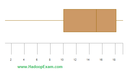
Consider the boxplot below.
Which of the following statements are true?
I. The distribution is skewed right.
II. The interquartile range is about 8.
III. The median is about 10.



1. I only
2. II only
3. Access Mostly Uused Products by 50000+ Subscribers
4. I and III
5. II and III

Ans : 2
Exp :

The correct answer is (B). Most of the observations are on the high end of the scale, so the distribution is skewed left. The interquartile range is indicated by the length of the box, which is 18 minus 10 or 8. And the median is indicated by the vertical line running through the middle of the box, which is roughly centered over 15. So the median is about 15.



Question : You are working with CISCO telephone department and
you need to model the failure rate of the telephone devices,
you chose the beta distribution to model the telephone failure rates,
with two variables a,b as shown in image why you decided to use beta distribution?



1. Because it has two parameters rather than one
2. Because it is conjugate to the binomial distribution
3. Access Mostly Uused Products by 50000+ Subscribers
4. Because it distribution ant bowl shape.
Ans : 2
Exp : Binomial distribution pops up in our problems daily, given that the number of occurrences k of events with probability p in a sequence of size n can be described as k=Binomial(n,p) Question that naturally arises in this context is - given observations of k and n , how do we estimate p ? One might say that simply computing p=kn should be enough, since that's both uniformly minimum variance and a maximum likelihood estimator. However, such estimator might be misleading when n is small (as anyone trying to estimate clickthrough rates from small number of impressions can testify). In this context, we can express our model as:
ki=Binomial(ni,pi)
pi=Beta(a,b),i=1...N
where N is total number of observations and a and b are parameters to be estimated. Such model is also called Empirical Bayes. Unlike traditional Bayes, in which we pull prior distribution and it's parameters out of the thin air, Empirical Bayes estimates prior parameters from the data.

The question is - what can we do ? One thing that naturally comes to mind is incorporating any prior knowledge about the distribution we might have. A wise choice for prior of binomial distribution is usually Beta distribution, not just because of it's convenience (given that it's conjugate prior), but also because of flexibility in incorporating different distribution shapes
In Bayesian probability theory, if the posterior distributions p(?|x) are in the same family as the prior probability distribution p(?), the prior and posterior are then called conjugate distributions, and the prior is called a conjugate prior for the likelihood function. For example, the Gaussian family is conjugate to itself (or self-conjugate) with respect to a Gaussian likelihood function: if the likelihood function is Gaussian, choosing a Gaussian prior over the mean will ensure that the posterior distribution is also Gaussian. This means that the Gaussian distribution is a conjugate prior for the likelihood which is also Gaussian. The concept, as well as the term "conjugate prior", was introduced by Howard Raiffa and Robert Schlaifer in their work on Bayesian decision theory. A similar concept had been discovered independently by George Alfred Barnard.
The following proposition states the relation between the Beta and the binomial distributions. Proposition suppose X is a random variable having a Beta distribution with parameters A and B. Let Y be another random variable such that its distribution conditional on X is a binomial distribution with parameters n and X. Then, the conditional distribution of X given Y=y is a Beta distribution with parameters A+y and B+n-y.
A simple model of hardware failure assumes that each device, independently and with equal probability, might fail over a short interval time. Given that probability, the number of failures in that interval can be modeled by the binomial distribution.
This probability is like a rate of failure and itself is not known and must be modeled. In terms of Bayesian theory, the likelihood function is from the binomial distribution. The prior and posterior distribution ought to be of the same form -- both represent knowledge about this rate of failure -- although with different estimates of that rate. A distribution with this relationship is called the conjugate prior. The conjugate prior for the binomial distribution is the beta distribution. Hence the beta distribution could usefully model knowledge about hardware failure rate.




Question :

Please select which of the following is not a supervised technique



1. Hierarchical Clustering
2. Linear Regression
3. Access Mostly Uused Products by 50000+ Subscribers
4. Naïve Bayesian Classifier
5. Decision Trees
Ans : 1
Exp : Supervised Learning
Linear Regression
Decision Trees
Naïve Bayesian Classifier
Artificial Neural Networks (Single-layer Perceptron)
k-Nearest Neighbour

Unsupervised Learning
Hierarchical Clustering
Agglomerative Clustering
Divisive Clustering



Question :

Map the followings

1. Clustering
2. Classification
3. Access Mostly Uused Products by 50000+ Subscribers


A. Build models to classify data into different categories
B. Build models to predict continuous data.
C. Find natural groupings and patterns in data.




1. 1-A,2-B,3-C
2. 1-B,2-C,3-A
3. Access Mostly Uused Products by 50000+ Subscribers
4. 1-B,2-A,3-C
Ans : 3
Exp : Classification
Build models to classify data into different categories.
Algorithms: support vector machine (SVM), boosted and bagged decision trees, k-nearest neighbor, Naïve Bayes, discriminant analysis, neural networks,

Regression
Build models to predict continuous data.
Algorithms: linear model, nonlinear model, regularization, stepwise regression, boosted and bagged decision trees, neural networks, adaptive neuro-fuzzy learning

Clustering
Find natural groupings and patterns in data.
Algorithms: k-means, hierarchical clustering, Gaussian mixture models, hidden Markov models, self-organizing maps, fuzzy c-means clustering, subtractive clustering,




Question :

Which of the following is not a correct application for the Classification?



1. credit scoring
2. tumor detection
3. Access Mostly Uused Products by 50000+ Subscribers
4. drug discovery
Ans : 4
Exp : Classification : Build models to classify data into different categories
credit scoring, tumor detection, image recognition
Regression: Build models to predict continuous data.
electricity load forecasting, algorithmic trading, drug discovery




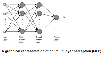
Question : The most common neural network model is the multi layer perceptron (MLP).
The perceptron is an algorithm for ____________ of an input into one of several possible non-binary outputs.
It is a type of linear classifier, i.e. a classification algorithm that makes its predictions based on a
linear predictor function combining a set of weights with the feature vector.




1. Pricipal Component Analysis
2. Simple Vector Machine
3. Access Mostly Uused Products by 50000+ Subscribers
4. Unsupervised learning
5. K-means clustering

Ans : 3
Exp : Neural Networks are an information processing technique based on the way biological nervous systems, such as the brain, process information. They resemble the human brain in the following two ways:A neural network acquires knowledge through learning. A neural network's knowledge is stored within inter-neuron connection strengths known as synaptic weights. Neural networks are being applied to an increasing large number of real world problems. Their primary advantage is that they can solve problems that are too complex for conventional technologies; problems that do not have an algorithmic solution or for which an algorithmic solution is too complex to be defined. In general, neural networks are well suited to problems that people are good at solving, but for which computers generally are not. These problems include pattern recognition and forecasting, which requires the recognition of trends in data.
The true power and advantage of neural networks lies in their ability to represent both linear and non-linear relationships and in their ability to learn these relationships directly from the data being modeled. Traditional linear models are simply inadequate when it comes to modeling data that contains non-linear characteristics.

The most common neural network model is the multi layer perceptron (MLP). This type of neural network is known as a supervised network because it requires a desired output in order to learn. The goal of this type of network is to create a model that correctly maps the input to the output using historical data so that the model can then be used to produce the output when the desired output is unknown.The MLP and many other neural networks learn using an algorithm called backpropagation. With backpropagation, the input data is repeatedly presented to the neural network. With each presentation the output of the neural network is compared to the desired output and an error is computed. This error is then fed back (backpropagated) to the neural network and used to adjust the weights such that the error decreases with each iteration and the neural model gets closer and closer to producing the desired output. This process is known as "training".In machine learning, the perceptron is an algorithm for supervised classification of an input into one of several possible non-binary outputs. It is a type of linear classifier, i.e. a classification algorithm that makes its predictions based on a linear predictor function combining a set of weights with the feature vector. The algorithm allows for online learning, in that it processes elements in the training set one at a time.

The perceptron is a binary classifier which maps its input (a real-valued vector) to an output value (a single binary value): The value of (0 or 1) is used to classify as either a positive or a negative instance, in the case of a binary classification problem. If is negative, then the weighted combination of inputs must produce a positive value greater than in order to push the classifier neuron over the 0 threshold. Spatially, the bias alters the position (though not the orientation) of the decision boundary. The perceptron learning algorithm does not terminate if the learning set is not linearly separable. If the vectors are not linearly separable learning will never reach a point where all vectors are classified properly. The most famous example of the perceptron's inability to solve problems with linearly nonseparable vectors is the Boolean exclusive-or problem. The solution spaces of decision boundaries for all binary functions and learning behaviors are studied in the reference. In the context of artificial neural networks, a perceptron is an artificial neuron using the Heaviside step function as the activation function. The perceptron algorithm is also termed the single-layer perceptron, to distinguish it from a multilayer perceptron, which is a misnomer for a more complicated neural network. As a linear classifier, the single-layer perceptron is the simplest feedforward neural network.




Question :

In which of the following scenerio, you can apply the Chi-Square test ?


1. Suppose you want to determine if certain types of products sell better in certain geographic locations than others.
2. Suppose you want to test if altering your product mix (% of upscale, mid-range and volume items, say) has impacted profits.
3. Access Mostly Uused Products by 50000+ Subscribers
4. Only 1 and 3
5. All 1,2 and 3

Ans : 5
Exp : Any business situation where you are essentially checking if one variable, X is related to, or independent of, another variable, Y. The use of chi-square test is indicated in any of the following business scenarios.

1. Suppose you want to determine if certain types of products sell better in certain geographic locations than others. A trivial example: the type of shoes sold in winter depends strongly on whether a retail outlet is located in the upper mid-west versus in the south. A slightly more complicated example would be to check if the type of gasoline sold in a neighborhood is indicative of the median income in the region. So variable X would be the type of gasoline and variable Y would be income ranges (e.g. less than 0k, 41k-50k, etc).
2. Suppose you want to test if altering your product mix (% of upscale, mid-range and volume items, say) has impacted profits. Here you could compare sales revenues of each product type before and after the change in product mix. Thus the categories in variable X would include all the product types and the categories in variable Y would include period 1 and period 2.
3. Access Mostly Uused Products by 50000+ Subscribers
No matter the business analytics problem, the chi-square test will find uses when you are trying to establish or invalidate that a relationship exists between two given business parameters that are categorical (or nominal) data types.





Question : Select the correct statement which applies to SVM (Support vector machine)


1. The SVM algorithm is a maximum margin classifier, and tries to pick a decision boundary that creates the widest margin between classes
2. SVMs are particularly better at multi-label classification
3. Access Mostly Uused Products by 50000+ Subscribers
4. Only 1 and 3
5. All 1,2 and 3

Ans : 1
Exp : You can use a support vector machine (SVM) when your data has exactly two classes. An SVM classifies data by finding the best hyperplane that separates all data points of one class from those of the other class. The best hyperplane for an SVM means the one with the largest margin between the two classes. Margin means the maximal width of the slab parallel to the hyperplane that has no interior data points.
The support vectors are the data points that are closest to the separating hyperplane; these points are on the boundary of the slab. The following figure illustrates these definitions, with + indicating data points of type 1, and - indicating data points of type -1.

The SVM algorithm is a maximum margin classifier, and tries to pick a decision boundary that creates the widest margin between classes, rather than just any boundary that separates the classes. This helps generalization to test data, since it is less likely to misclassify points near the decision boundary, as the boundary maintains a large margin from training examples.

SVMs are not particularly better at multi-label clasification. Linear separability is not required for either classification technique, and does not relate directly to an advantage of SVMs. SVMs are not particularly more suited to low dimensional data.



Question : When you have "The test set you have are very high-dimensional spaces, Memory-intensive and kind of annoying to run , tune, dense,
and contain examples close to decision boundary learned from the training set" then which is the best technique from the below you consider

1. Support vector machine
2. Logistic regression
3. Access Mostly Uused Products by 50000+ Subscribers
4. 1 and 3
5. 1 and 2
Ans : 1
Exp : You can use a support vector machine (SVM) when your data has exactly two classes. An SVM classifies data by finding the best hyperplane that separates all data points of one class from those of the other class. The best hyperplane for an SVM means the one with the largest margin between the two classes. Margin means the maximal width of the slab parallel to the hyperplane that has no interior data points.
The support vectors are the data points that are closest to the separating hyperplane; these points are on the boundary of the slab. The following figure illustrates these definitions, with + indicating data points of type 1, and - indicating data points of type -1.

The SVM algorithm is a maximum margin classifier, and tries to pick a decision boundary that creates the widest margin between classes, rather than just any boundary that separates the classes. This helps generalization to test data, since it is less likely to misclassify points near the decision boundary, as the boundary maintains a large margin from training examples. SVMs are not particularly better at multi-label clasification. Linear separability is not required for either classification technique, and does not relate directly to an advantage of SVMs. SVMs are not particularly more suited to low dimensional data. Advantages of Naive Bayes: Super simple, you're just doing a bunch of counts. If the NB conditional independence assumption actually holds, a Naive Bayes classifier will converge quicker than discriminative models like logistic regression, so you need less training data. And even if the NB assumption doesn't hold, a NB classifier still often performs surprisingly well in practice. A good bet if you want to do some kind of semi-supervised learning, or want something embarrassingly simple that performs pretty well.
Advantages of Logistic Regression: Lots of ways to regularize your model, and you don't have to worry as much about your features being correlated, like you do in Naive Bayes. You also have a nice probabilistic interpretation, unlike decision trees or SVMs, and you can easily update your model to take in new data (using an online gradient descent method), again unlike decision trees or SVMs. Use it if you want a probabilistic framework (e.g., to easily adjust classification thresholds, to say when you're unsure, or to get confidence intervals) or if you expect to receive more training data in the future that you want to be able to quickly incorporate into your model.
Advantages of Decision Trees: Easy to interpret and explain (for some people -- I'm not sure I fall into this camp). Non-parametric, so you don't have to worry about outliers or whether the data is linearly separable (e.g., decision trees easily take care of cases where you have class A at the low end of some feature x, class B in the mid-range of feature x, and A again at the high end). Their main disadvantage is that they easily overfit, but that's where ensemble methods like random forests (or boosted trees) come in. Plus, random forests are often the winner for lots of problems in classification (usually slightly ahead of SVMs, I believe), they're fast and scalable, and you don't have to worry about tuning a bunch of parameters like you do with SVMs, so they seem to be quite popular these days.
Advantages of SVMs: High accuracy, nice theoretical guarantees regarding overfitting, and with an appropriate kernel they can work well even if you're data isn't linearly separable in the base feature space. Especially popular in text classification problems where very high-dimensional spaces are the norm. Memory-intensive and kind of annoying to run and tune, though, so I think random forests are starting to steal the crown.
To go back to the particular question of logistic regression vs. decision trees (which I'll assume to be a question of logistic regression vs. random forests) and summarize a bit: both are fast and scalable, random forests tend to beat out logistic regression in terms of accuracy, but logistic regression can be updated online and gives you useful probabilities. And since you're at Square (not quite sure what an inference scientist is, other than the embodiment of fun) and possibly working on fraud detection: having probabilities associated to each classification might be useful if you want to quickly adjust thresholds to change false positive/false negative rates, and regardless of the algorithm you choose, if your classes are heavily imbalanced (as often happens with fraud), you should probably resample the classes or adjust your error metrics to make the classes more equal.




Question : Assume some output variable "y" is a linear combination of some independent input variables "X" plus some independent noise "e".
The way the independent variables are combined is defined by a parameter vector B
y=XB+e
Also assume that the noise term "e" is drawn from a standard Normal distribution.
e = N(0,I)
For some estimate of the model parameters B , the models prediction errors/residuals "e"
are the difference between the model prediction and the observed ouput values
e=y-XB
So what would be this B value



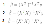
1.
2.
3. Access Mostly Uused Products by 50000+ Subscribers
Ans : 1
Exp : This is the standard solution of the normal equations for linear regression



Question : Assume some output variable "y" is a linear combination of some independent input variables "P" plus some independent noise "e".
The way the independent variables are combined is defined by a parameter vector Q
y=PQ+e where X is an m x n matrix, Q is a vector of n unknowns, and e is a vector of m values.
Assuming that m is not equal to n and the columns of X are linearly independent, which expression correctly solves for Q?


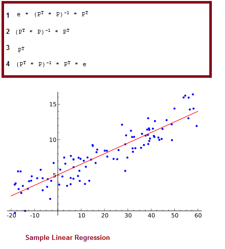
1.
2.
3. Access Mostly Uused Products by 50000+ Subscribers
4.
Ans : 4
Exp : In statistics, linear regression is an approach for modeling the relationship between a scalar dependent variable y and one or more explanatory variables (or independent variable) denoted X. The case of one explanatory variable is called simple linear regression. For more than one explanatory variable, the process is called multiple linear regression.[1] (This term should be distinguished from multivariate linear regression, where multiple correlated dependent variables are predicted, rather than a single scalar variable.)[2]

In linear regression, data are modeled using linear predictor functions, and unknown model parameters are estimated from the data. Such models are called linear models.[3] Most commonly, linear regression refers to a model in which the conditional mean of y given the value of X is an affine function of X. Less commonly, linear regression could refer to a model in which the median, or some other quantile of the conditional distribution of y given X is expressed as a linear function of X. Like all forms of regression analysis, linear regression focuses on the conditional probability distribution of y given X, rather than on the joint probability distribution of y and X, which is the domain of multivariate analysis.

Linear regression was the first type of regression analysis to be studied rigorously, and to be used extensively in practical applications.[4] This is because models which depend linearly on their unknown parameters are easier to fit than models which are non-linearly related to their parameters and because the statistical properties of the resulting estimators are easier to determine.

Linear regression has many practical uses. Most applications fall into one of the following two broad categories:

If the goal is prediction, or forecasting, or reduction, linear regression can be used to fit a predictive model to an observed data set of y and X values. After developing such a model, if an additional value of X is then given without its accompanying value of y, the fitted model can be used to make a prediction of the value of y.
Given a variable y and a number of variables X1, ..., Xp that may be related to y, linear regression analysis can be applied to quantify the strength of the relationship between y and the Xj, to assess which Xj may have no relationship with y at all, and to identify which subsets of the Xj contain redundant information about y.
Linear regression models are often fitted using the least squares approach, but they may also be fitted in other ways, such as by minimizing the "lack of fit" in some other norm (as with least absolute deviations regression), or by minimizing a penalized version of the least squares loss function as in ridge regression (L2-norm penalty) and lasso (L1-norm penalty). Conversely, the least squares approach can be used to fit models that are not linear models. Thus, although the terms "least squares" and "linear model" are closely linked, they are not synonymous.This is the standard solution of the normal equations for linear regression. Because A is not square, you cannot simply take its inverse.



Question : Select the correct statement from the below
1. Regularization is designed to eliminate variables that are simply noise and are not related to the underlying predictor variables.
2. Both L1 and L2 require a penalty weight (some floating-point number >= 0.0) to be added to the objective function that is optimized for the model
3. Access Mostly Uused Products by 50000+ Subscribers
4. Both L1 and L2 will effectively zero-out the coefficients of variables that are not related to the predictor.
5. L1 leads to more parsimonious models (i.e., fewer variables are included), which makes for a simpler model and is generally better



1. 1,2,3,4
2. 2,3,4,5
3. Access Mostly Uused Products by 50000+ Subscribers
4. 1,2,4,5
5. 1,2,4,5

Ans : 4
Exp : Regularization is designed to eliminate variables that are simply noise and are not related to the underlying predictor variables. It is a computational form of variable selection (which is also called "feature selection"), and both L1 and L2 require a penalty weight (some floating-point number >= 0.0) to be added to the objective function that is optimized for the model. The L1 penalty is an absolute value function that isn't differentiable, while the L2 penalty is a squared-loss function that can be differentiated.
Both L1 and L2 will effectively zero-out the coefficients of variables that are not related to the predictor. The key difference between them is that when several of the independent variables are correlated with one another, L1 will choose exactly one of those features into include in the model, whereas L2 will make the coefficients of the correlated variables roughly equal to one another. For this reason, L1 leads to more parsimonious models (i.e., fewer variables are included), which makes for a simpler model and is generally better. The reason that L2 is used in many contexts (including most distributed regression models of the form that we would build on, say, Hadoop) is because a distributed L1-regularization problem is effectively equal to a distributed L2 regularization problem, and the L2 regularization problem is usually easier to solve.
The takeaway here is: L1 regularization is better, but it typically requires that your model fits on a single machine. L2 regularization still has some (but not all) of the advantages of L1, but its main benefit is that it works across many machines.




Question : Select the correct statements from belwo.
1. Primary advantage of L2 regularization over L1 regularization for variable selection is "It is easier to parallelize"
2. L1 regularization is better, but it typically requires that your model fits on a single machine.
3. Access Mostly Uused Products by 50000+ Subscribers
4. L2 regularization is better, but it typically requires that your model fits on a single machine.
5. L1 regularization still has some (but not all) of the advantages of L1, but its main benefit is that it works across many machines



1. 1,2,3,4
2. 2,3,4,5
3. Access Mostly Uused Products by 50000+ Subscribers
4. 2,3,4
5. 1,3,4

Ans : 3
Explanation:Regularization is designed to eliminate variables that are simply noise and are not related to the underlying predictor variables. It is a computational form of variable selection (which is also called "feature selection"), and both L1 and L2 require a penalty weight (some floating-point number >= 0.0) to be added to the objective function that is optimized for the model. The L1 penalty is an absolute value function that isn't differentiable, while the L2 penalty is a squared-loss function that can be differentiated.
Both L1 and L2 will effectively zero-out the coefficients of variables that are not related to the predictor. The key difference between them is that when several of the independent variables are correlated with one another, L1 will choose exactly one of those features into include in the model, whereas L2 will make the coefficients of the correlated variables roughly equal to one another. For this reason, L1 leads to more parsimonious models (i.e., fewer variables are included), which makes for a simpler model and is generally better. The reason that L2 is used in many contexts (including most distributed regression models of the form that we would build on, say, Hadoop) is because a distributed L1-regularization problem is effectively equal to a distributed L2 regularization problem, and the L2 regularization problem is usually easier to solve.
The takeaway here is: L1 regularization is better, but it typically requires that your model fits on a single machine. L2 regularization still has some (but not all) of the advantages of L1, but its main benefit is that it works across many machines




Question : Distributed L-regularization problem is effectively equal to a distributed L regularization problem,
and the L2 regularization problem is usually easier to solve.


1. True
2. False
Ans : 1
Regularization is designed to eliminate variables that are simply noise and are not related to the underlying predictor variables. It is a computational form of variable selection (which is also called "feature selection"), and both L1 and L2 require a penalty weight (some floating-point number >= 0.0) to be added to the objective function that is optimized for the model. The L1 penalty is an absolute value function that isn't differentiable, while the L2 penalty is a squared-loss function that can be differentiated.

Both L1 and L2 will effectively zero-out the coefficients of variables that are not related to the predictor. The key difference between them is that when several of the independent variables are correlated with one another, L1 will choose exactly one of those features into include in the model, whereas L2 will make the coefficients of the correlated variables roughly equal to one another. For this reason, L1 leads to more parsimonious models (i.e., fewer variables are included), which makes for a simpler model and is generally better. The reason that L2 is used in many contexts (including most distributed regression models of the form that we would build on, say, Hadoop) is because a distributed L1-regularization problem is effectively equal to a distributed L2 regularization problem, and the L2 regularization problem is usually easier to solve.

The takeaway here is: L1 regularization is better, but it typically requires that your model fits on a single machine. L2 regularization still has some (but not all) of the advantages of L1, but its main benefit is that it works across many machines.




Question : You are building a classifier off of a very high-dimensional data set
similar to shown in the image with 5000 variables (lots of columns, not that many rows).
It can handle both dense and sparse input. Which technique is most suitable, and why?




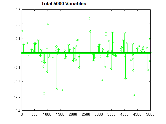
1. Logistic regression with L1 regularization, to prevent overfitting
2. Naive Bayes, because Bayesian methods act as regularlizers
3. Access Mostly Uused Products by 50000+ Subscribers
4. Random forest, because it is an ensemble method
Ans : 1 Exp : Logistic regression is widely used in machine learning for classification problems. It is well-known that regularization is required to avoid over-fitting, especially when there is a only small number of training examples, or when there are a large number of parameters to be learned. In particular, L1 regularized logistic regression is often used for feature selection, and has been shown to have good generalization performance in the presence of many irrelevant features. (Ng 2004; Goodman 2004) Unregularized logistic regression is an unconstrained con-vex optimization problem with a continuously differentiable objective function. As a consequence, it can be solved fairly efficiently with standard convex optimization methods, such as Newton's method or conjugate gradient. However, adding the L1 regularization makes the optimization problem com-putationally more expensive to solve. If the L1 regulariza-tion is enforced by an L1 norm constraint on the parameLogistic regression is a classifier, and L1 regularization tends to produce models that ignore dimensions of the input that are not predictive. This is particularly useful when the input contains many dimensions. k-nearest neighbors classification is also a classification technique, but relies on notions of distance. In a high-dimensional space, most every data point is "far" from others (the curse of dimensionality) and so these techniques break down. Naive Bayes is not inherently regularizing. Random forests represent an ensemble method, but an ensemble method is not necessarily more suitable to high-dimensional data. Practically, I think the biggest reasons for regularization are 1) to avoid overfitting by not generating high coefficients for predictors that are sparse. 2) to stabilize the estimates especially when there's collinearity in the data.
1) is inherent in the regularization framework. Since there are two forces pulling each other in the objective function, if there's no meaningful loss reduction, the increased penalty from the regularization term wouldn't improve the overall objective function. This is a great property since a lot of noise would be automatically filtered out from the model.
To give you an example for 2), if you have two predictors that have same values, if you just run a regression algorithm on it since the data matrix is singular, your beta coefficients will be Inf if you try to do a straight matrix inversion. But if you add a very small regularization lambda to it, you will get stable beta coefficients with the coefficient values evenly divided between the equivalent two variables.
For the difference between L1 and L2, the following graph demonstrates why people bother to have L1 since L2 has such an elegant analytical solution and is so computationally straightforward. Regularized regression can also be represented as a constrained regression problem (since they are Lagrangian equivalent). The implication of this is that the L1 regularization gives you sparse estimates. Namely, in a high dimensional space, you got mostly zeros and a small number of non-zero coefficients. This is huge since it incorporates variable selection to the modeling problem. In addition, if you have to score a large sample with your model, you can have a lot of computational savings since you don't have to compute features(predictors) whose coefficient is 0. I personally think L1 regularization is one of the most beautiful things in machine learning and convex optimization. It is indeed widely used in bioinformatics and large scale machine learning for companies like Facebook, Yahoo, Google and Microsoft.



Question : Consider the following confusion matrix for a data set with out of , instances positive:

In this case, Precision = 50%, Recall = 83%, Specificity = 95%, and Accuracy = 95%.
Select the correct statement




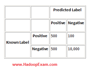
1. Precision is low, which means the classifier is predicting positives best
2. Precision is low, which means the classifier is predicting positives poorly
3. Access Mostly Uused Products by 50000+ Subscribers
4. 1 and 3
5. 2 and 3
Ans : 5
Exp : In this case, Precision = 50%, Recall = 83%, Specificity = 95%, and Accuracy = 95%. In this case, Precision is low, which means the classifier is predicting positives poorly. However, the three other measures seem to suggest that this is a good classifier. This just goes to show that the problem domain has a major impact on the measures that should be used to evaluate a classifier within it, and that looking at the 4 simple cases presented is not sufficient.



Question : From the , sample books you have based on the title, prepface, author, publisher you want to classify and used trained a binary classifier
and after running against your test set (13000 Sample books data) . It correctly classified 5000 books as belonging to Software Books and 4000 books
are not software books. And also incorrectly classified 1000 books as belonging to software books and 3000 books not belonging to software book.
What is the recall for your trained classifier on this test dataset?



1. 0.500
2. 0.600
3. Access Mostly Uused Products by 50000+ Subscribers
4. 0.750
5. 1.00
Ans : 3 Exp : In pattern recognition and information retrieval with binary classification, precision (also called positive predictive value) is the fraction of retrieved instances that are relevant, while recall (also known as sensitivity) is the fraction of relevant instances that are retrieved. Both precision and recall are therefore based on an understanding and measure of relevance. Suppose a program for recognizing dogs in scenes from a video identifies 7 dogs in a scene containing 9 dogs and some cats. If 4 of the identifications are correct, but 3 are actually cats, the program's precision is 4/7 while its recall is 4/9. When a search engine returns 30 pages only 20 of which were relevant while failing to return 40 additional relevant pages, its precision is 20/30 = 2/3 while its recall is 20/60 = 1/3. In statistics, if the null hypothesis is that all and only the relevant items are retrieved, absence of type I and type II errors corresponds respectively to maximum precision (no false positive) and maximum recall (no false negative). The above pattern recognition example contained 7 - 4 = 3 type I errors and 9 - 4 = 5 type II errors. Precision can be seen as a measure of exactness or quality, whereas recall is a measure of completeness or quantity. In simple terms, high precision means that an algorithm returned substantially more relevant results than irrelevant, while high recall means that an algorithm returned most of the relevant results. 5000 books were software books, and correctly identified as such (true positives). 3000 other books were software books but not identified as such (false negatives). Recall = TP / (TP+FN) = 5000 / (5000 + 3000) = 0.625
sensitivity or true positive rate (TPR)
eqv. with hit rate, recall
{TPR} = {TP} / P = {TP} / ({TP}+{FN})
specificity (SPC) or True Negative Rate
{SPC} = {TN} / N = {TN} / ({FP} + {TN})
precision or positive predictive value (PPV)
{PPV} = {TP} / ({TP} + {FP})
negative predictive value (NPV)
{NPV} = {TN} / ({TN} + {FN})
fall-out or false positive rate (FPR)
{FPR} = {FP} / N = {FP} / ({FP} + {TN})
false discovery rate (FDR)
{FDR} = {FP} / ({FP} + {TP}) = 1 - {PPV}
false negative rate (FNR)
{FNR} = {FN} / ({FN} + {TP}) = 1 - {TPR}


Question : Let's say we want to insert the strings "foo" and "bar" into a Bloom filter that is bits wide, and we have two hash functions.
1. Compute the two hashes of "foo", and get the values 1 and 6.
2. Set bits 1 and 6 in the bit array.
3. Access Mostly Uused Products by 50000+ Subscribers
4. Set bits 6 and 3 in the bit array.

Suppose we now want to query the Bloom filter, to see whether the value "baz" are present.
Compute the two hashes of "baz", and get the values 1 and 3

So after that we will report




1. true positive
2. false positive
3. Access Mostly Uused Products by 50000+ Subscribers
4. false negative
Ans : 2
Exp : Suppose we now want to query the Bloom filter, to see whether the values "quux" and "baz" are present.
1. Compute the two hashes of "quux", and get the values 4 and 0.
2. Check bit 4 in the bit array. It is not set, so "quux" cannot be present. We do not need to check bit 0.
3. Access Mostly Uused Products by 50000+ Subscribers
4. Check bit 1 in the bit array. It is set, as is bit 3, so we say that "baz" is present even though it is not. We have reported a false positive.




Question : You have created a bloom filter as shown in the figure. An example of a Bloom filter, representing the set { x, y, z }.
The colored arrows show the positions in the bit array that each set element is mapped to. The element w is not in the set { x, y, z },
because it hashes to one bit-array position containing 0. For this figure, m = 18 and k = 3. You now hash the 19th element from the
data set into the Bloom filter, and you find that the new item hashes to two empty locations and two non-empty locations.
Which statement describes the probability that the item already in the existing dataset.?


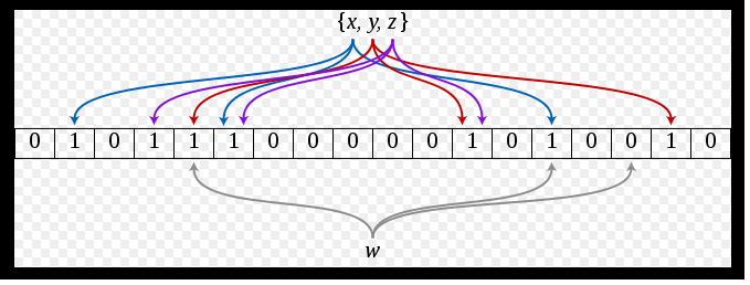
1. There is a 100% probability
2. There is a 0% probability
3. Access Mostly Uused Products by 50000+ Subscribers
4. There is a 25% probability
Ans : 2
Exp : Many questions in counting can be answered by a simple yes or no. Have we seen user X before? Can we trust that IP? Does Melville use the word "banana" in Moby Dick? Each of these questions can be answered by building a set, then querying whether or not a given input value is a member of the set. We could hash each word in Moby Dick into a hash table, for example, then hash "banana" to see if we get any collisions.

Often, only the yes or no is important, and the value about which the question is asked is irrelevant. In that case, we can use a sketching data structure called a bloom filter to get the answer without storing anything extra.

Enter Bloom Filters : The bloom filter data structure is effectively a hash table where collisions are ignored and each element added to the table is hashed by some number k hash functions. There is one major difference, however: a bloom filter does not store the hashed keys. Instead, it has a bit array as its underlying data structure; each key is remembered by flipping on all of the bits the k functions map it to. Querying the filter will report that a given key is either "probably in" (yes) or "definitely not in" (no) the set. For many applications, that's all the information that we need.

Bloom filters have two primary operations: insertion and membership querying. In general, removal is not supported since it would introduce the possibility of false negatives. Suppose we now want to query the Bloom filter, to see whether the values "quux" and "baz" are present.
1. Compute the two hashes of "quux", and get the values 4 and 0.
2. Check bit 4 in the bit array. It is not set, so "quux" cannot be present. We do not need to check bit 0.
3. Access Mostly Uused Products by 50000+ Subscribers
4. Check bit 1 in the bit array. It is set, as is bit 3, so we say that "baz" is present even though it is not. We have reported a false positive.

If an item hashes to any empty locations in a Bloom filter, the item has not been seen before.
Bloom filters are designed for situations where a false negative is a Very Bad Thing and a false positive is acceptable.

For example, suppose that you are making a web browser and have a known blacklist of scam websites. Your blacklist is massive - in the hundreds of gigabytes - so you can't ship it with the browser. However, you can store it on your own servers. In that case, you could ship the browser with a Bloom filter of an appropriate size that holds all the URLs. Before visiting a site, you look it up in the filter. Then, if you get a "no" answer, you're guaranteed that the URL is not blacklisted and can just visit the site. If you get a "yes" answer, the site might be evil, so you can have the browser call up your main server to get the real answer. The fact that you can save a huge number of calls to the server here without ever sacrificing accuracy is important.

The cache idea is similar to this setup. You can query the filter to see if the page is in the cache. If you get a "no" answer, you're guaranteed it's not cached and can do an expensive operation to pull the data from the main source. Otherwise, you can then check the cache to see if it really is there. In rare instances you might need to check the cache, see that it isn't there, then pull from the main source, but you will never accidentally miss something really in cache.




Question : You are having a variable x,y and z and need to sample a -dimensional unit-cube. To properly sample any given dimension out of
x,y and z , you wil be having 10 points. How many points do you need in order to sample the complete this 3-dimensional unit cube?

1. 10
2. 100
3. Access Mostly Uused Products by 50000+ Subscribers
4. 10000
Ans : 3
Exp : This problem is an example of the curse of dimensionality.
To adequately sample a single dimension requires only 10 points or a sample distance of 0.1.
To achieve the same coverage in 3 dimensions, you need 10 points in each dimension, which means 10 power 3 which is 1000 points need to be sampled. The curse of dimensionality refers to various phenomena that arise when analyzing and organizing data in high-dimensional spaces (often with hundreds or thousands of dimensions) that do not occur in low-dimensional settings such as the three-dimensional physical space of everyday experience.

There are multiple phenomena referred to by this name in domains such as numerical analysis, sampling, combinatorics, machine learning, data mining and databases. The common theme of these problems is that when the dimensionality increases, the volume of the space increases so fast that the available data become sparse. This sparsity is problematic for any method that requires statistical significance. In order to obtain a statistically sound and reliable result, the amount of data needed to support the result often grows exponentially with the dimensionality. Also organizing and searching data often relies on detecting areas where objects form groups with similar properties; in high dimensional data however all objects appear to be sparse and dissimilar in many ways which prevents common data organization strategies from being efficient. The "curse of dimensionality" is not a problem of high-dimensional data, but a joint problem of the data and the algorithm being applied. It arises when the algorithm does not scale well to high-dimensional data, typically due to needing an amount of time or memory that is exponential in the number of dimensions of the data.

When facing the curse of dimensionality, a good solution can often be found by changing the algorithm, or by pre-processing the data into a lower-dimensional form. For example, the notion of intrinsic dimension refers to the fact that any low-dimensional data space can trivially be turned into a higher-dimensional space by adding redundant (e.g. duplicate) or randomized dimensions, and in turn many high-dimensional data sets can be reduced to lower-dimensional data without significant information loss. This is also reflected by the effectiveness of dimension reduction methods such as principal component analysis in many situations. Algorithms that are based on distance functions or nearest neighbor search can also work robustly on data having many spurious dimensions, depending on the statistics of those dimensions.



Question : . Select the correct statement which applies to Language Modeling
1. It can be used in speech recognition system
2. It cannot help discriminate between similar sounding words
3. Access Mostly Uused Products by 50000+ Subscribers
4. It can help case and punctuation restoration


1. 1,2,3
2. 2,3,4
3. Access Mostly Uused Products by 50000+ Subscribers
4. 1,2,3,4
Ans : 3
Exp : Why are LMs interesting?
o Important component of a speech recognition system
- Helps discriminate between similar sounding words
- Helps reduce search costs
o In statistical machine translation, a language model characterizes the
target language, captures fluency
o For selecting alternatives in summarization, generation
o Text classification (style, reading level, language, topic, . . . )
o Language models can be used for more than just words
- letter sequences (language identification)
- speech act sequence modeling
- case and punctuation restoration

Language model tells you which strings are more likely
Used where there is natural language input
Voice Recognition
Handwriting-to-text
Transliteration schemes
Machine translation





Question : Which of the following is a best example of natural language processing, language model:



1. Converting audio output out of new words.
2. It is useful for predicting the probability of a sequence of words/or upcoming words
3. Access Mostly Uused Products by 50000+ Subscribers
4. Creating the Images out of words, for captcha creation.


Ans : 2 Exp :Why are LMs interesting? o Important component of a speech recognition system - Helps discriminate between similar sounding words - Helps reduce search costs o In statistical machine translation, a language model characterizes the target language, captures fluency
o For selecting alternatives in summarization, generation o Text classification (style, reading level, language, topic, . . . ) o Language models can be used for more than just words - letter sequences (language identification) - speech act sequence modeling - case and punctuation restoration

Language model tells you which strings are more likely
Used where there is natural language input
Voice Recognition
Handwriting-to-text
Transliteration schemes
Machine translation
A statistical language model assigns a probability to a sequence of m words P(w_1,\ldots,w_m) by means of a probability distribution. Having a way to estimate the relative likelihood of different phrases is useful in many natural language processing applications. Language modeling is used in speech recognition, machine translation, part-of-speech tagging, parsing, handwriting recognition, information retrieval and other applications.

In speech recognition, the computer tries to match sounds with word sequences. The language model provides context to distinguish between words and phrases that sound similar. For example, in American English, the phrases "recognize speech" and "wreck a nice beach" are pronounced the same but mean very different things. These ambiguities are easier to resolve when evidence from the language model is incorporated with the pronunciation model and the acoustic model.

Language models are used in information retrieval in the query likelihood model. Here a separate language model is associated with each document in a collection. Documents are ranked based on the probability of the query Q in the document's language model P(Q|M_d). Commonly, the unigram language model is used for this purpose"otherwise known as the bag of words model.

Data sparsity is a major problem in building language models. Most possible word sequences will not be observed in training. One solution is to make the assumption that the probability of a word only depends on the previous n words. This is known as an N-gram model or unigram model when n=1.
In natural language processing, a language model is a method of calculating the probability of a sentence or a sequence of words. An n-gram model is a common example. The goal of Statistical Language Modeling is to build a statistical language model that can estimate the distribution of natural language as accurate as possible. A statistical language model (SLM) is a probability distribution P(s) over strings S that attempts to reflect how frequently a string S occurs as a sentence. By expressing various language phenomena in terms of simple parameters in a statistical model, SLMs provide an easy way to deal with complex natural language in computer. The original (and is still the most important) application of SLMs is speech recognition, but SLMs also play a vital role in various other natural language applications as diverse as machine translation, part-of-speech tagging, intelligent input method and Text To Speech system.



Question : In probability theory and information theory, the mutual information (MI) or (formerly) transinformation of two random variables is a measure of
the variables' mutual dependence. Not limited to real-valued random variables like the correlation coefficient, MI is more general and determines how similar
the joint distribution p(X,Y) is to the products of factored marginal distribution p(X)p(Y). MI is the expected values of the pointwise mutual information (PMI).
The most common unit of measurement of mutual information is the bit. Correlation between sets of data is a measure of how well they are related. The most common
measure of correlation in stats is the Pearson Correlation. The full name is the Pearson Product Moment Correlation or PPMC. It shows the linear relationship
between two sets of data. In simple terms, it answers the question, Can I draw a line graph to represent the data? What are the advantages of the mutual
information over the Pearson correlation for text classification problems?

1. The mutual information gives more meaningful information than Pearson Correlation
2. The mutual information can signal non-linear relationships between the dependent and independent variables.
3. Access Mostly Uused Products by 50000+ Subscribers
4. The mutual information doesn't assume that the variables are normally distributed as Pearson Correlation does.

Ans : 3
Exp : In probability theory and information theory, the mutual information (MI) or (formerly) transinformation of two random variables is a measure of the variables' mutual dependence. Not limited to real-valued random variables like the correlation coefficient, MI is more general and determines how similar the joint distribution p(X,Y) is to the products of factored marginal distribution p(X)p(Y). MI is the expected values of the pointwise mutual information (PMI). The most common unit of measurement of mutual information is the bit. Correlation between sets of data is a measure of how well they are related. The most common measure of correlation in stats is the Pearson Correlation. The full name is the Pearson Product Moment Correlation or PPMC. It shows the linear relationship between two sets of data. In simple terms, it answers the question, Can I draw a line graph to represent the data? A linear scaling of the input variables (that may be caused by a change of units for the measurements) is sufficient to modify the PCA results. Feature selection methods that are sufficient for simple distributions of the patterns belonging to different classes can fail in classification tasks with complex decision boundaries. In addition, methods based on a linear dependence (like the correlation) cannot take care of arbitrary relations between the pattem coordinates and the different classes. On the contrary, the mutual information can measure arbitrary relations between variables and it does not depend on transformations acting on the different variables.
This item concerns itself with feature selection for a text classification problem and references mutual information criteria. Mutual information is a bit more sophisticated than just selecting based on the simple correlation of two numbers because it can detect non-linear relationships that will not be identified by the correlation. Whenever possible, mutual information is a better feature selection technique than correlation.
: Mutual information is a quantification of the dependency between random variables. It is sometimes contrasted with linear correlation since mutual information captures nonlinear dependence.
Correlation analysis provides a quantitative means of measuring the strength of a linear relationship between two vectors of data. Mutual information is essentially the measure of how much "knowledge" one can gain of a certain variable by knowing the value of another variable.




Question : Select the correct Hashing Trick Application

1. dimensionality reduction
2. sparsification
3. Access Mostly Uused Products by 50000+ Subscribers
4. cross-product features
5. multi-task learning



1. 1,2,3
2. 2,3,4
3. Access Mostly Uused Products by 50000+ Subscribers
4. 1,2,3,4
5. All 1,2,3,4,5

Ans : 5
Exp : Let's say we want to design a function v = phi(x), which from a d-dimensional vector x = (x(1), x(2), ..., x(d)) outputs a new m-dimensional vector v, with m either greater or smaller than d. In other words, phi can be used either for reducing dimensionality of x (d > m) or for sparsifying x (m > d).
One way to do so is to use a hash function h to map x(1) to v(h(1)), x(2) to v(h(2)), ..., x(d) to v(h(d)). Hash functions are functions which, from an arbitrary integer input, can output an integer in a specified range. Good hash functions should have uniform output and obey the avalanche effect: a small perturbation in the input must result in a great change in the output. This ensures that any dimension in x will be mapped to a random dimension in v. Note that this will typically results in collisions (two dimensions in x can be mapped to the same dimension in v) but in practice, this won't affect performance if m is big enough.
In document classification, documents are typically transformed to vectors in the bag-of-word representation. The problem with that is that you don't know the dimensionality of your vectors until you've made an entire pass over your dataset. Fortunately there exist hash functions which take string as input. We can thus map words to a dimension in v as we go. I think this is why it is called the hashing trick: similarly to the kernel trick, v = phi(x) never needs to be computed explicitly. The ability to transform documents as you go is very useful in online algorithms such as SGD. Vowpal Wabbit uses something like 2^26 for m.
I've also seen hash functions used to automatically generate cross-product features. If you have a hash function which gives you an integer from two integers, i.e. i = h(a,b), you can now map the combined feature x(a) * x(b) to v(i). Cross-product features can be useful to model the interactions between features.
The paper "Feature Hashing for Large Scale Multitask Learning" (Weinberger et al., ICML09) also shows how to use the hashing trick for multi-task learning. For example, in spam filtering, since each user typically receives different kinds of spam, it would be nice if we could use one binary classifier per user. This is an example of multi-task learning since each task is related. Obviously it would require massive amounts of storage to store the weight vector of each classifier. The authors show that it is possible to use one hash function per user (as well as one global function) to combine the different users into one feature space. This is a recommended reading as it also covers the background on the hashing trick.
To summarize some of the applications:
odimensionality reduction
osparsification
obag-of-words on the fly
ocross-product features
omulti-task learning





Question : Select the correct statement which applies to K-Mean Clustering?

1. When the numbers of data are not so many, initial grouping will determine the cluster significantly.
2. The number of cluster, K, must be determined before hand.
3. Access Mostly Uused Products by 50000+ Subscribers
4. We never know which attribute contributes more to the grouping process since we assume that each attribute has the same weight.


1. 1,2
2. 2,3
3. Access Mostly Uused Products by 50000+ Subscribers
4. 2,3,4
5. All 1,2,3 and 4

Ans : 5
Exp : What are the weaknesses of K-Mean Clustering?
Similar to other algorithm, K-mean clustering has many weaknesses:
- When the numbers of data are not so many, initial grouping will determine the cluster significantly.
- The number of cluster, K, must be determined beforehand.
- We never know the real cluster, using the same data, if it is inputted in a different way may produce different cluster if the number of data is a few.
- We never know which attribute contributes more to the grouping process since we assume that each attribute has the same weight.
One way to overcome those weaknesses is to use K-mean clustering only if there are available many data.




Question : Suppose you have several objects and each object have several attributes and you want
to classify the objects based on the attributes, then you can apply K-Mean Clustering?



1. True
2. False

Ans : 1
Exp :

There are a lot of applications of the K-mean clustering, range from unsupervised learning of neural network,
Pattern recognitions, Classification analysis, Artificial intelligent, image processing, machine vision, etc. In principle, you have several objects and each object have several attributes and you want to classify the objects based on the attributes, then you can apply this algorithm.



Question : Select the correct statement which applies to unsupervised learning



1. The more tightly you fit the data, the less stable the model will be.
2. A good approach is to set a stability threshold and select the model that achieves the lowest cost above the stability threshold
3. Access Mostly Uused Products by 50000+ Subscribers
4. 1 and 2
5. 1 and 3

Ans : 5
Exp : There is a tradeoff between cost and stability in unsupervised learning. The more tightly you fit the data, the less stable the model will be, and vice versa. The idea is to find a good balance with more weight given to the cost. Typically a good approach is to set a stability threshold and select the model that achieves the lowest cost above the stability threshold.



Question : The goal in unsupervised learning may be to discover groups of similar examples within the data (like all the books in
same group), where it is called clustering, or to determine the distribution of data within the input space, known as density estimation,
or to project the data from a high-dimensional space down to two or three dimensions for the purpose of visualization. Which of the following
will describe the quality of the model with the given cost of clustering and its stability of the model in unsupervised learning.
1. Cost of clustring : How good is the data for model e.g. for given vector points
( The cost is the squared distance between all the points to their closest cluster center. )

2. Stability of Model : If you run the your analytics on the cluster again and again using the same data whether it produce the same result or not.
Stability of the results across different runs is considered to be an asset of the algorithm.


1. If the cluster is low cost then it is subject to a stability constraint
2. If the cost is low for clustring model.
3. Access Mostly Uused Products by 50000+ Subscribers
4. If it has most stable clustering

Ans : 1
Exp : The goal in unsupervised learning may be to discover groups of similar examples within the data (like all the books in same group), where it is called clustering, or to determine the distribution of data within the input space, known as density estimation, or to project the data from a high-dimensional space down to two or three dimensions for the purpose of visualization. There is a tradeoff between cost and stability in unsupervised learning. The more tightly you fit the data, the less stable the model will be, and vice versa. The idea is to find a good balance with more weight given to the cost. Typically a good approach is to set a stability threshold and select the model that achieves the lowest cost above the stability threshold. An experimental comparison with the stability of the standard k-means algorithm was carried out for k from 2 to 20. The results revealed that ensembles are generally more stable, markedly so for larger k. To establish whether stability can serve as a cluster validity index, we first looked at the relationship between stability and accuracy with respect to the number of clusters, k. We found that such a relationship strongly depends on the data set, varying from almost perfect positive correlation (0.97, for the glass data) to almost perfect negative correlation (-0.93, for the crabs data). We propose a new combined stability index to be the sum of the pairwise individual and ensemble stabilities. This index was found to correlate better with the ensemble accuracy. Following the hypothesis that a point of stability of a clustering algorithm corresponds to a structure found in the data, we used the stability measures to pick the number of clusters. The combined stability index gave best results




Question : Select the correct objective of PCA



1. To discover or to reduce the dimensionality of the data set.
2. To identify new meaningful underlying variables
3. Access Mostly Uused Products by 50000+ Subscribers
4. NOne of 1 and 2


Ans : 3
Exp : Principal component analysis (PCA) involves a mathematical procedure that transforms a number of (possibly) correlated variables into a (smaller) number of uncorrelated variables called principal components. The first principal component accounts for as much of the variability in the data as possible, and each succeeding component accounts for as much of the remaining variability as possible.
Objectives of principal component analysis
To discover or to reduce the dimensionality of the data set.
To identify new meaningful underlying variables.




Question : PCA is a method to transform a multi-variable data set by a rotation. A rotation is found so that the first axis corresponding to the first
component is rotated to the direction where the variance of the data set is greatest. The next component will then be the direction perpendicular to the first
with the most variance and so on. Figure show an example with a two-variable data set where the new axes are drawn. Which line represent PCA ?

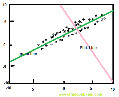
1. Pink
2. Green
3. Access Mostly Uused Products by 50000+ Subscribers

Ans : 2
Exp :PCA is a method to transform a multi-variable data set by a rotation. A rotation is found so that the first axis corresponding to the first component is rotated to the direction where the variance of the data set is greatest. The next component will then be the direction perpendicular to the first with the most variance and so on. Figure 6 show an example with a two-variable data set where the new axes are drawn.Principal component analysis (PCA) involves a mathematical procedure that transforms a number of (possibly) correlated variables into a (smaller) number of uncorrelated variables called principal components. The first principal component accounts for as much of the variability in the data as possible, and each succeeding component accounts for as much of the remaining variability as possible. The first principal component corresponds to the greatest variance in the data. The green line is evidently this first principal component, because if we project the data onto the blue line, the data is more spread out (higher variance) than if projected onto any other line, including the pink one. In this application the purpose of PCA is to reduce the number of channels to analyze. In the example it is obvious that most of the variance in the data set is along the first principal component. Assuming that variance equals information contents, one can extract almost all information in the measurement from just one channel.
The EEG recordings available here have seven channels. Because of the way signals propagate from a source in the brain to the electrodes, large signals will be measured at all electrodes and hence the channels will be highly correlated. The primary interest here is the large signals, as they relative easy can be extracted without too much noise. Therefore PCA is an appropriate tool to reduce the number of channels to analyze. The way it is used here is referred to in the literature as “spatial PCA�.
The concept of eigenvalues and eigenvectors has to be introduced before describing how to find the transformation, which gives the principal components.




Question : You have a large x data matrix DM.
You decide you want to perform dimension reduction/clustering on your data and have decided to use the QR decomposition.
A is 6 x 6 lower triangular , B is 6 x 6 unitary , C is 12 x 12 unitary , D is 6 x 12 diagonal , E is 12 x 12 orthogonal
F is 12 x 12 diagonal , G is 12 x 12 invertible , H is 6 x 6 upper triangular , I is 12 x 12 upper triangular
What represents the QR decomposition of the 12 x 12 matrix DM?


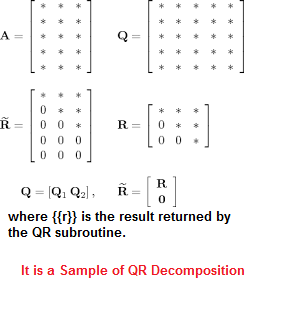
1. DM = B D C
2. DM = G F G power -1
3. Access Mostly Uused Products by 50000+ Subscribers
4. DM = A H
5. DM = E I


Ans : 5
Exp : In linear algebra, a QR decomposition (also called a QR factorization) of a matrix is a decomposition of a matrix A into a product A = QR of an orthogonal matrix Q and an upper triangular matrix R. QR decomposition is often used to solve the linear least squares problem, and is the basis for a particular eigenvalue algorithm, the QR algorithm. If A has n linearly independent columns, then the first n columns of Q form an orthonormal basis for the column space of A. More specifically, the first k columns of Q form an orthonormal basis for the span of the first k columns of A for any n>=k>=1. The fact that any column k of A only depends on the first k columns of Q is responsible for the triangular form of R. The basic goal of the QR decomposition is to factor a matrix as a product of two matrices (traditionally called , hence the name of this factorization). Each matrix has a simple structure which can be further exploited in dealing with, say, linear equations. The QR decomposition is nothing else than the Gram-Schmidt procedure applied to the columns of the matrix, and with the result expressed in matrix form. The QR decomposition decomposes a matrix into an orthogonal and upper triangular matrix, by definition. Of the two upper triangular matrices, only R has the correct n x n dimension. The basic goal of the QR decomposition is to factor a matrix as a product of two matrices (traditionally called Q,R, hence the name of this factorization). Each matrix has a simple structure which can be further exploited in dealing with, say, linear equations. The QR decomposition is nothing else than the Gram-Schmidt procedure applied to the columns of the matrix, and with the result expressed in matrix form. Consider a m times n matrix A = (a_1,ldots,a_n), with each a_i in mathbf{R}^m a column of A.




Question :. Singular values give valuable information whether a square matrix is singular.
A square matrix is non-singular (i.e. have inverse) if and only if


1. all its singular values are different from zero.
2. all its singular values are different from ones
3. Access Mostly Uused Products by 50000+ Subscribers
4. all its singular values are ones.


Ans : 1
Exp : Singular values give valuable information whether a square matrix is singular. A square matrix is non-singular (i.e. have inverse) if and only if all its singular values are different from zero.


Question : What kind of decomposition this image is depicting.



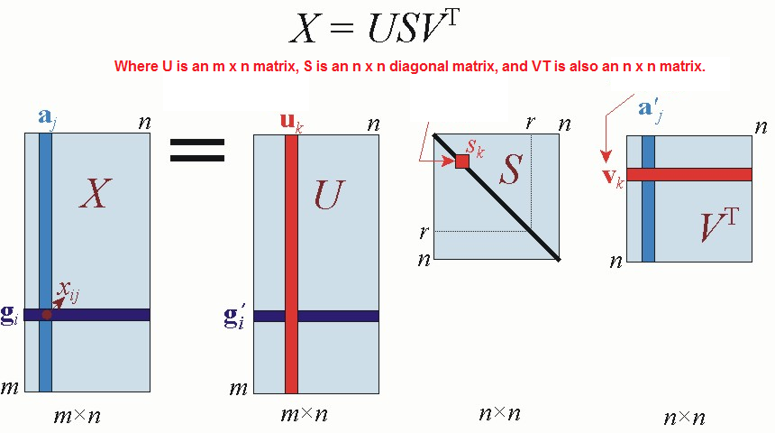
1. Lower Upper decomposition
2. Singular value decomposition
3. Access Mostly Uused Products by 50000+ Subscribers
4. QR decomposition

Ans : 2
Exp :In numerical analysis, LU decomposition (where 'LU' stands for 'Lower Upper', and also called LU factorization) factors a matrix as the product of a lower triangular matrix and an upper triangular matrix. The product sometimes includes a permutation matrix as well. The LU decomposition can be viewed as the matrix form of Gaussian elimination. Computers usually solve square systems of linear equations using the LU decomposition, and it is also a key step when inverting a matrix, or computing the determinant of a matrix. Singular value decomposition (SVD) is a means of decomposing a a matrix into a product of three simpler matrices. In this way it is related to other matrix decompositions such as eigen decomposition, principal components analysis (PCA), and non-negative matrix factorization (NNMF).
This is the canonical definition of the SVD, where a matrix is decomposed into the product of two orthonormal matrices, with a diagonal matrix in between. This does not match the decomposition provided by any of the other options. One of the challenges of bioinformatics is to develop effective ways to analyze global gene expression data. A rigorous approach to gene expression analysis must involve an up-front characterization of the structure of the data. In addition to a broader utility in analysis methods, singular value decomposition (SVD) and principal component analysis (PCA) can be valuable tools in obtaining such a characterization. SVD and PCA are common techniques for analysis of multivariate data, and gene expression data are well suited to analysis using SVD/PCA. A single microarray Endnote experiment can generate measurements for thousands, or even tens of thousands of genes. Present experiments typically consist of less than ten assays, but can consist of hundreds (Hughes et al., 2000). Gene expression data are currently rather noisy, and SVD can detect and extract small signals from noisy data.

The goal of this chapter is to provide precise explanations of the use of SVD and PCA for gene expression analysis, illustrating methods using simple examples. We describe SVD methods for visualization of gene expression data, representation of the data using a smaller number of variables, and detection of patterns in noisy gene expression data. In addition, we describe the mathematical relation between SVD analysis and Principal Component Analysis (PCA) when PCA is calculated using the covariance matrix, enabling our descriptions to apply equally well to either method. Our aims are 1) to provide descriptions and examples of the application of SVD methods and interpretation of their results; 2) to establish a foundation for understanding previous applications of SVD to gene expression analysis; and 3) to provide interpretations and references to related work that may inspire new advances.





Question : KMeans is a clustering algorithm. Its purpose is to partition a set of vectors into K groups
that cluster around common mean vector. This can also be thought as approximating the input each of the input
vector with one of the means, so the clustering process finds, in principle, the best dictionary or codebook to
vector quantize the data.What is the best way to ensure that this algorithm will find a good clustering of a input
collection of vectors?



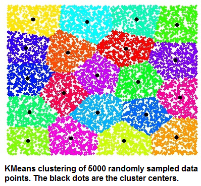
1. Choose the initial centroids so that they are having average distance among all the distances.
2. Run at least log(N) iterations of Lloyd's algorithm, where N is the number of observations in the data set
3. Access Mostly Uused Products by 50000+ Subscribers
4. Choose the initial centroids so that they are far away from each other

Ans : 4
Exp : The k-means algorithm takes as input the number of clusters to generate, k, and a set of observation vectors to cluster. It returns a set of centroids, one for each of the k clusters. An observation vector is classified with the cluster number or centroid index of the centroid closest to it.

A vector v belongs to cluster i if it is closer to centroid i than any other centroids. If v belongs to i, we say centroid i is the dominating centroid of v. The k-means algorithm tries to minimize distortion, which is defined as the sum of the squared distances between each observation vector and its dominating centroid. Each step of the k-means algorithm refines the choices of centroids to reduce distortion. The change in distortion is used as a stopping criterion: when the change is lower than a threshold, the k-means algorithm is not making sufficient progress and terminates. One can also define a maximum number of iterations.

Since vector quantization is a natural application for k-means, information theory terminology is often used. The centroid index or cluster index is also referred to as a "code" and the table mapping codes to centroids and vice versa is often referred as a "code book". The result of k-means, a set of centroids, can be used to quantize vectors. Quantization aims to find an encoding of vectors that reduces the expected distortion. This question is about the properties that make k-means an effective clustering heuristic, which primarily deal with ensuring that the initial centers are far away from each other. This is how modern k-means algorithms like k-means++ guarantee that with high probability Lloyd's algorithm will find a clustering within a constant factor of the optimal possible clustering for each k.
All routines expect obs to be a M by N array where the rows are the observation vectors. The codebook is a k by N array where the i'th row is the centroid of code word i. The observation vectors and centroids have the same feature dimension. As an example, suppose we wish to compress a 24-bit color image (each pixel is represented by one byte for red, one for blue, and one for green) before sending it over the web. By using a smaller 8-bit encoding, we can reduce the amount of data by two thirds. Ideally, the colors for each of the 256 possible 8-bit encoding values should be chosen to minimize distortion of the color. Running k-means with k=256 generates a code book of 256 codes, which fills up all possible 8-bit sequences. Instead of sending a 3-byte value for each pixel, the 8-bit centroid index (or code word) of the dominating centroid is transmitted. The code book is also sent over the wire so each 8-bit code can be translated back to a 24-bit pixel value representation. If the image of interest was of an ocean, we would expect many 24-bit blues to be represented by 8-bit codes. If it was an image of a human face, more flesh tone colors would be represented in the code book.k-means clustering is a method of vector quantization, originally from signal processing, that is popular for cluster analysis in data mining. k-means clustering aims to partition n observations into k clusters in which each observation belongs to the cluster with the nearest mean, serving as a prototype of the cluster. This results in a partitioning of the data space into Voronoi cells. The problem is computationally difficult (NP-hard); however, there are efficient heuristic algorithms that are commonly employed and converge quickly to a local optimum. These are usually similar to the expectation-maximization algorithm for mixtures of Gaussian distributions via an iterative refinement approach employed by both algorithms. Additionally, they both use cluster centers to model the data; however, k-means clustering tends to find clusters of comparable spatial extent, while the expectation-maximization mechanism allows clusters to have different shapes





Question : Which of the following is a correct properties of Mahalanobis distance


1. It accounts for the fact that the variances in each direction are different.
2. It accounts for the covariance between variables.
3. Access Mostly Uused Products by 50000+ Subscribers
4. Only 1 and 3
5. All 1,2 and 3


Ans : 5
Exp : : You can use the probability contours to define the Mahalanobis distance. The Mahalanobis distance has the following properties:
o It accounts for the fact that the variances in each direction are different.
o It accounts for the covariance between variables.
o It reduces to the familiar Euclidean distance for uncorrelated variables with unit variance.





Question : The Mahalanobis distance is a descriptive statistic that provides a relative measure of a
data point's distance (residual) from a common point. It is a unitless measure introduced by P. C. Mahalanobis in 1936.
The Mahalanobis distance is used to identify and gauge similarity of an unknown sample set to a known one.
It differs from Euclidean distance in that it takes into account the correlations of the data set and is scale-invariant.
In other words, it has a multivariate effect size. Or The Mahalanobis distance is a variation on the Euclidean distance
that incorporates the inverse of the covariance matrix between dimensions into the distance calculation.
In what class of problems is this distance metric most useful?

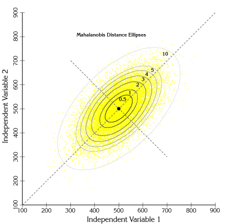
1. Sentiment analysis
2. Singular value decomposition
3. Access Mostly Uused Products by 50000+ Subscribers
4. Outlier detection


Ans : 4 Exp : The Mahalanobis distance is a measure of the distance between a point P and a distribution D, introduced by P. C. Mahalanobis in 1936.[1] It is a multi-dimensional generalization of the idea of measuring how many standard deviations away P is from the mean of D. This distance is zero if P is at the mean of D, and grows as P moves away from the mean: Along each principal component axis, it measures the number of standard deviations from P to the mean of D. If each of these axes is rescaled to have unit variance, then Mahalanobis distance corresponds to standard Euclidean distance in the transformed space. Mahalanobis distance is thus unitless and scale-invariant, and takes into account the correlations of the data set. Mahalanobis distance is a normalized measure of distance that takes into account the fact that clusters of points may not be similarly distributed along all axes. It's most useful for identifying points that are notably further away from a set of reference points than the other points in the dataset. Consider the problem of estimating the probability that a test point in N-dimensional Euclidean space belongs to a set, where we are given sample points that definitely belong to that set. Our first step would be to find the average or center of mass of the sample points. Intuitively, the closer the point in question is to this center of mass, the more likely it is to belong to the set.

However, we also need to know if the set is spread out over a large range or a small range, so that we can decide whether a given distance from the center is noteworthy or not. The simplistic approach is to estimate the standard deviation of the distances of the sample points from the center of mass. If the distance between the test point and the center of mass is less than one standard deviation, then we might conclude that it is highly probable that the test point belongs to the set. The further away it is, the more likely that the test point should not be classified as belonging to the set.

This intuitive approach can be made quantitative by defining the normalized distance between the test point and the set to be {x - mu}/sigma . By plugging this into the normal distribution we can derive the probability of the test point belonging to the set.

The drawback of the above approach was that we assumed that the sample points are distributed about the center of mass in a spherical manner. Were the distribution to be decidedly non-spherical, for instance ellipsoidal, then we would expect the probability of the test point belonging to the set to depend not only on the distance from the center of mass, but also on the direction. In those directions where the ellipsoid has a short axis the test point must be closer, while in those where the axis is long the test point can be further away from the center.

Putting this on a mathematical basis, the ellipsoid that best represents the set's probability distribution can be estimated by building the covariance matrix of the samples. The Mahalanobis distance is simply the distance of the test point from the center of mass divided by the width of the ellipsoid in the direction of the test point.



Question : Lloyd's algorithm algorithm is based on the observation that,
while jointly optimizing clusters
and assignment is difficult, optimizing one given the other is easy.
In what way can Hadoop be used to improve the performance
of Lloyd's algorithm for k-means clustering on large data sets?

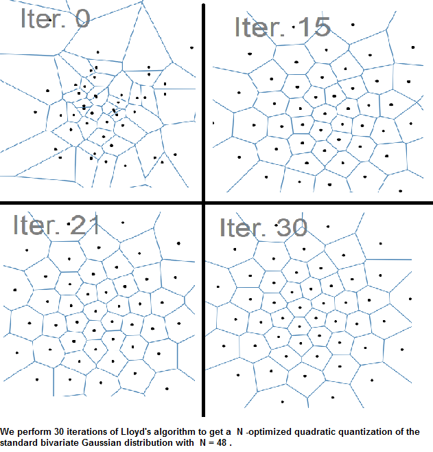
1. It reduces the number of iterations
2. It is capable of distributing the updates of the cluster centroids
3. Access Mostly Uused Products by 50000+ Subscribers
4. None of the above

Ans : 2
Exp : The most common K-means method is Lloyd's algorithm . This algorithm is based on the observation that, while jointly optimizing clusters and assignment is difficult, optimizing one given the other is easy. Lloyd's algorithm alternates the steps:
1. Quantization. Each point x i is reassigned to the center c q j closer to it. This requires finding for each point the closest among K other points, which is potentially slow.
2. Center estimation. Each center c q is updated to minimize its average distances to the points assigned to it. It is easy to show that the best center is the mean or median of the points, respectively if the l 2 or l 1 norm is considered.
When running Lloyd's algorithm on Hadoop, the centroid assignments are done in the map phase, and the calculation of new centroids is done in the reduce phase. Running on Hadoop has no impact on the convergence of the algorithm or its numerical stability. Lloyd's algorithm is designed for running on points in Euclidean spaces.





Question : This is the most popular method for data approximation by straight lines and planes, and for dimensionality reduction.
Projecting a multi-dimensional dataset onto which vector has the greatest variance, ________________

1. first principal component
2. first eigenvector
3. Access Mostly Uused Products by 50000+ Subscribers
4. second eigenvector
5. not enough information given to answer

Ans : 1 Exp : The method based on principal component analysis (PCA) evaluates the features according to the projection of the largest eigenvector of the correlation matrix on the initial dimensions, the method based on Fisher's linear discriminant analysis evaluates.them according to the magnitude of the components of the discriminant vector. The first principal component corresponds to the greatest variance in the data, by definitinon. If we project the data onto the first principal component line, the data is more spread out (higher variance) than if projected onto any other line, including other principal components.
Principal component analysis (PCA) involves a mathematical procedure that transforms a number of (possibly) correlated variables into a (smaller) number of uncorrelated variables called principal components. The first principal component accounts for as much of the variability in the data as possible, and each succeeding component accounts for as much of the remaining variability as possible.
1. Objectives of principal component analysis
To discover or to reduce the dimensionality of the data set. To identify new meaningful underlying variables.
2. How to start : We assume that the multi-dimensional data have been collected in a TableOfReal data matrix, in which the rows are associated with the cases and the columns with the variables. Traditionally, principal component analysis is performed on the symmetric Covariance matrix or on the symmetric Correlation matrix. These matrices can be calculated from the data matrix. The covariance matrix contains scaled sums of squares and cross products. A correlation matrix is like a covariance matrix but first the variables, i.e. the columns, have been standardized. We will have to standardize the data first if the variances of variables differ much, or if the units of measurement of the variables differ. You can standardize the data in the TableOfReal by choosing Standardize columns.
To perform the analysis, we select the TabelOfReal data matrix in the list of objects and choose To PCA. This results in a new PCA object in the list of objects.
We can now make a scree plot of the eigenvalues, Draw eigenvalues... to get an indication of the importance of each eigenvalue. The exact contribution of each eigenvalue (or a range of eigenvalues) to the "explained variance" can also be queried: Get fraction variance accounted for.... You might also check for the equality of a number of eigenvalues: Get equality of eigenvalues....
3. Access Mostly Uused Products by 50000+ Subscribers
4. Getting the principal components : Principal components are obtained by projecting the multivariate datavectors on the space spanned by the eigenvectors. This can be done in two ways: 1. Directly from the TableOfReal without first forming a PCA object: To Configuration (pca).... You can then draw the Configuration or display its numbers. 2. Select a PCA and a TableOfReal object together and choose To Configuration.... In this way you project the TableOfReal onto the PCA's eigenspace.


Question : Apache Sqoop(TM) is a tool designed for efficiently transferring bulk data between Apache Hadoop and structured datastores such as relational
databases. You use Sqoop to import a table from your RDBMS into HDFS. You have configured to use 3 mappers in Sqoop, to controll the number of
parallelism and memory in use. Once the table import is finished, you notice that total 7 Mappers have run, there are 7 output files in HDFS,
and 4 of the output files is empty. Why?


1. The table does not have a numeric primary key
2. The table does not have a primary key
3. Access Mostly Uused Products by 50000+ Subscribers
4. The table does not have a unique key




Question : Using Apache Sqoop you can import the data to



1. Apache Hive
2. Apache HBase
3. Access Mostly Uused Products by 50000+ Subscribers
4. Only 1 and 3
5. All 1,2 and 3

Ans : 5
Exp : : Apache Sqoop can be used to import data from any relational DB into HDFS, Hive or HBase.
To import data into HDFS, use the sqoop import command and specify the relational DB table and connection parameters:

sqoop import --connect "JDBC connection string" --table "tablename" --username "username" --password "password"
This will import the data and store it as a CSV file in a directory in HDFS. To import data into Hive, use the sqoop import command and specify the option 'hive-import'.

sqoop import --connect "JDBC connection string" --table "tablename" --username "username" --password "password" --hive-importThis will import the data into a Hive table with the approproate data types for each column.


Question : You dont have dataset as of now with you, but you are planning to use Hive table for your data to be processed by downstream system.
Hence downstream needs table definition in advance and they are fine with the empty data table in Hive. So you created following table definition
Under HADOOPEXAM database.
CREATE TABLE USERPROFILES(USER_NAME STRING, USER_ID INT, USER_ZIPCODE INT);
Now downstream is ready with the end to end set up. You have to feed the data directly in this Hive table. And data volume is huge almost 500GB
As data volume is high you can not fire Insert statement, you already have data in csv format. So in which directory of HDFS you need to dump this
csv file assume all the default setting Hive has.

1. /user/hive/warehouse/HADOOPEXAM/USERPROFILES
2. /user/hive/warehouse/HADOOPEXAM.db/USERPROFILES
3. Access Mostly Uused Products by 50000+ Subscribers
4. /user/hive/HADOOPEXAM.db/USERPROFILES
5. /user/hive/warehouse/HADOOPEXAM USERPROFILES

Ans : 2
Exp : Databases in Hive
The Hive concept of a database is essentially just a catalog or namespace of tables. However, they are very useful for larger clusters with multiple teams and users, as a way of avoiding table name collisions. It's also common to use databases to organize production tables into logical groups. If you don't specify a database, the default database is used. The simplest syntax for creating a database is shown in the following example:
hive> CREATE DATABASE financials; Hive will throw an error if financials already exists. You can suppress these warnings with this variation:
hive> CREATE DATABASE IF NOT EXISTS financials; While normally you might like to be warned if a database of the same name already exists, the IF NOT EXISTS clause is useful for scripts that should create a database on-the-fly, if necessary, before proceeding.
You can also use the keyword SCHEMA instead of DATABASE in all the database-related commands. At any time, you can see the databases that already exist as follows:
hive> SHOW DATABASES; default financials
hive> CREATE DATABASE human_resources; hive> SHOW DATABASES;
default financials human_resources
If you have a lot of databases, you can restrict the ones listed using a regular expression, a concept we'll explain in LIKE and RLIKE, if it is new to you. The following example lists only those databases that start with the letter h and end with any other characters (the .* part):
hive> SHOW DATABASES LIKE 'h.*'; human_resources Hive will create a directory for each database. Tables in that database will be stored in subdirectories of the database directory. The exception is tables in the default database, which doesn't have its own directory. The database directory is created under a top-level directory specified by the property hive.metastore.warehouse.dir, which we discussed in Local Mode Configuration and Distributed and Pseudodistributed Mode Configuration. Assuming you are using the default value for this property, /user/hive/warehouse, when the financials database is created, Hive will create the directory /user/hive/warehouse/financials.db. Note the .db extension. You can override this default location for the new directory as shown in this example:
hive> CREATE DATABASE financials > LOCATION '/my/preferred/directory'; You can add a descriptive comment to the database, which will be shown by the DESCRIBE DATABASE (database) command. hive> CREATE DATABASE financials > COMMENT 'Holds all financial tables'; hive> DESCRIBE DATABASE financials;
financials Holds all financial tables hdfs://master-server/user/hive/warehouse/financials.db Note that DESCRIBE DATABASE also shows the directory location for the database. In this example, the URI scheme is hdfs. For a MapR installation, it would be maprfs. For an Amazon Elastic MapReduce (EMR) cluster, it would also be hdfs, but you could set hive.metastore.warehouse.dir to use Amazon S3 explicitly (i.e., by specifying s3n://bucketname/… as the property value). You could use s3 as the scheme, but the newer s3n is preferred. In the output of DESCRIBE DATABASE, we're showing master-server to indicate the URI authority, in this case a DNS name and optional port number (i.e., server:port) for the "master node" of the filesystem (i.e., where the NameNode service is running for HDFS). If you are running in pseudo-distributed mode, then the master server will be localhost. For local mode, the path will be a local path, file:///user/hive/warehouse/financials.db. If the authority is omitted, Hive uses the master-server name and port defined by the property fs.default.name in the Hadoop configuration files, found in the $HADOOP_HOME/conf directory. To be clear, hdfs:///user/hive/warehouse/financials.db is equivalent to hdfs://master-server/user/hive/warehouse/financials.db, where master-server is your master node's DNS name and optional port. For completeness, when you specify a relative path (e.g., some/relative/path), Hive will put this under your home directory in the distributed filesystem (e.g., hdfs:///user/user-name) for HDFS. However, if you are running in local mode, your current working directory is used as the parent of some/relative/path.When you create a database named HADOOPEXAM in Hive, that creates a subdirectory of Hive's warehouse directory named HADOOPEXAM.db. All tables are placed in subdirectories of HADOOPEXAM.db; those subdirectory names are the names of the tables



Question :. For HadoopExam.com user profiles you need to analyze roughly ,, JPEG files of all the.
Each file is no more than 3kB. Now you want to group the files into a single archive.
Which of the following file formats should you select to build your archive?


1. JAR
2. SequenceFiles
3. Access Mostly Uused Products by 50000+ Subscribers
4. ZIP
5. Avro

Ans : 5

Exp : Apache Avro is a data serialization system. Avro provides: Rich data structures. A compact, fast, binary data format. A container file, to store persistent data. Remote procedure call (RPC). Simple integration with dynamic languages. Code generation is not required to read or write data files nor to use or implement RPC protocols. Code generation as an optional optimization, only worth implementing for statically typed languages.
Schemas : Avro relies on schemas. When Avro data is read, the schema used when writing it is always present. This permits each datum to be written with no per-value overheads, making serialization both fast and small. This also facilitates use with dynamic, scripting languages, since data, together with its schema, is fully self-describing. When Avro data is stored in a file, its schema is stored with it, so that files may be processed later by any program. If the program reading the data expects a different schema this can be easily resolved, since both schemas are present. When Avro is used in RPC, the client and server exchange schemas in the connection handshake. (This can be optimized so that, for most calls, no schemas are actually transmitted.) Since both client and server both have the other's full schema, correspondence between same named fields, missing fields, extra fields, etc. can all be easily resolved.
Avro schemas are defined with JSON . This facilitates implementation in languages that already have JSON libraries.
Comparison with other systems : Avro provides functionality similar to systems such as Thrift, Protocol Buffers, etc. Avro differs from these systems in the following fundamental aspects. Dynamic typing: Avro does not require that code be generated. Data is always accompanied by a schema that permits full processing of that data without code generation, static datatypes, etc. This facilitates construction of generic data-processing systems and languages.
Untagged data: Since the schema is present when data is read, considerably less type information need be encoded with data, resulting in smaller serialization size.
No manually-assigned field IDs: When a schema changes, both the old and new schema are always present when processing data, so differences may be resolved symbolically, using field names. Apache Avro, Avro, Apache, and the Avro and Apache logos are trademarks of The Apache Software Foundation.The two formats that are best suited to merging small files into larger archives for processing in Hadoop are Avro and SequenceFiles. Avro has Ruby bindings; SequenceFiles are only supported in Java. JSON, TIFF, and MPEG are not appropriate formats for archives. JSON is also not an appropriate format for image data.



Question :
Select the correct statement which applies to calculate the probabilities in log space?



1. It is more efficient to divide probabilities in log space
2. It is more efficient to multiply probabilities in log space
3. Access Mostly Uused Products by 50000+ Subscribers
4. To avoid underflow
5. 3 and 4